
What Does Seasonal Decomposition Separate, and How Do You Read the Parts?
Updated October 2026
Split a series into a trend, a pattern that repeats, and what is left. Then a busy December is not mistaken for growth.
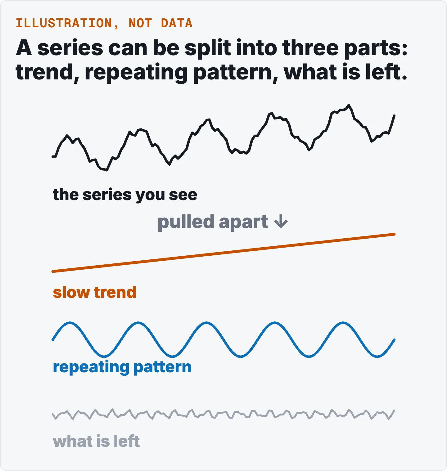
Seasonal decomposition splits a series into a trend, a pattern that repeats on a calendar, and what is left [1]. Our framing: that way a busy December is not taken for growth. The trend is the slow movement. The season part occurs over a fixed and known period, such as the month or the day of the week. The rest is what is left over [1]. With the three apart you can ask three plain questions. Which way is the level moving, how strong is the repeating pattern, and what is odd about this month. This page covers the three parts, additive versus multiplicative, how the pattern is found, how its strength is measured, the traps, and what our free tool does.
Also on this topic: the business version, on a shop's monthly sales and the version for analysts, on carbon dioxide readings.
The answer first: three parts, three questions
Split a series into its three parts and you can ask three plain questions. Which way is the level moving? How strong is the pattern that repeats? What is odd once the pattern is out?
| Part | What it is | The question it answers |
|---|---|---|
| Trend | The slow movement. | Which way is the level moving? |
| Season | The pattern that repeats on a calendar. | How strong is the repeating pattern? |
| Rest | Whatever is left over. | What is unusual? |
What this means for you
- A busy month is not growth until you have taken the pattern out. A December high may be only the calendar.
- Read the trend, the pattern and the rest one at a time. Each answers its own question.
What seasonal decomposition is: the three parts
A series can be read as trend, seasonal, cyclical and irregular parts [1]. This page uses the three-part view, because the cyclical part is often merged into the trend. The trend is the long-term progression of the series. It does not have to be a straight line [1]. The seasonal part occurs over a fixed and known period, such as the quarter of the year, the month or the day of the week [1]. The irregular part, which we call the rest, is the random influence that is left once the others are removed [1].
The cyclical part is a different thing. It is repeated but non-periodic fluctuation [1]. Our example: a business cycle has no fixed interval. It is not seasonal. The trend line may contain cyclical swings [1]. The two are sometimes merged into one trend-cycle [1].
Additive vs multiplicative: two ways to join the parts
There are two ways to put the parts back together. In an additive decomposition the series is the season part plus the trend plus the rest. It is best suited when the size of the season swings does not vary with the level of the series [2]. In a multiplicative decomposition the series is the season part times the trend times the rest. It is better suited when the variation looks proportional to the level [2].
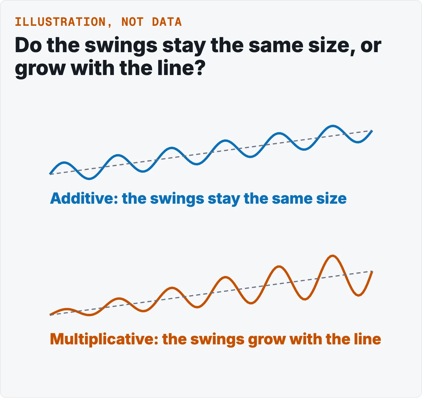
Our reading of that test: you can often decide by looking at the line. If the swings stay about the same size as the line climbs, additive is the natural fit. If they widen as the line climbs, multiplicative is [2].
How the pattern is found
STL, short for Seasonal and Trend decomposition using Loess (a way of drawing a smooth line through scattered points), has advantages over the classical method [3]. It handles any season period, it lets the season component change over time under the user's control. It lets the user set how smooth the trend is [3]. When specified, it can also be robust to outliers, which means odd points have less pull. Odd points then have less effect on the trend and season estimates, though they still show up in the rest [3][4].
How strong is the pattern?
One measure of strength compares the leftover to the pattern. Variance means how much numbers spread out, and detrended data is the series with the trend taken out. On the detrended data, strength is 1 minus the variance of the rest divided by the variance of the season part and the rest together, with a floor of 0 [6]. A value close to 0 means almost no seasonality. A value close to 1 means the variance of the rest is much smaller than that of the season part plus the rest [6]. The source gives the range and those two readings. It gives no cut between weak and strong. This page offers none as general.
Traps
STL is additive only. For multiplicative swings, take logs first. STL also does not automatically handle trading-day or calendar variation [3]. Our advice, not a sourced rule. Adjust for the number of days or trading days in each month before decomposing. A short month is not read as a weak one.
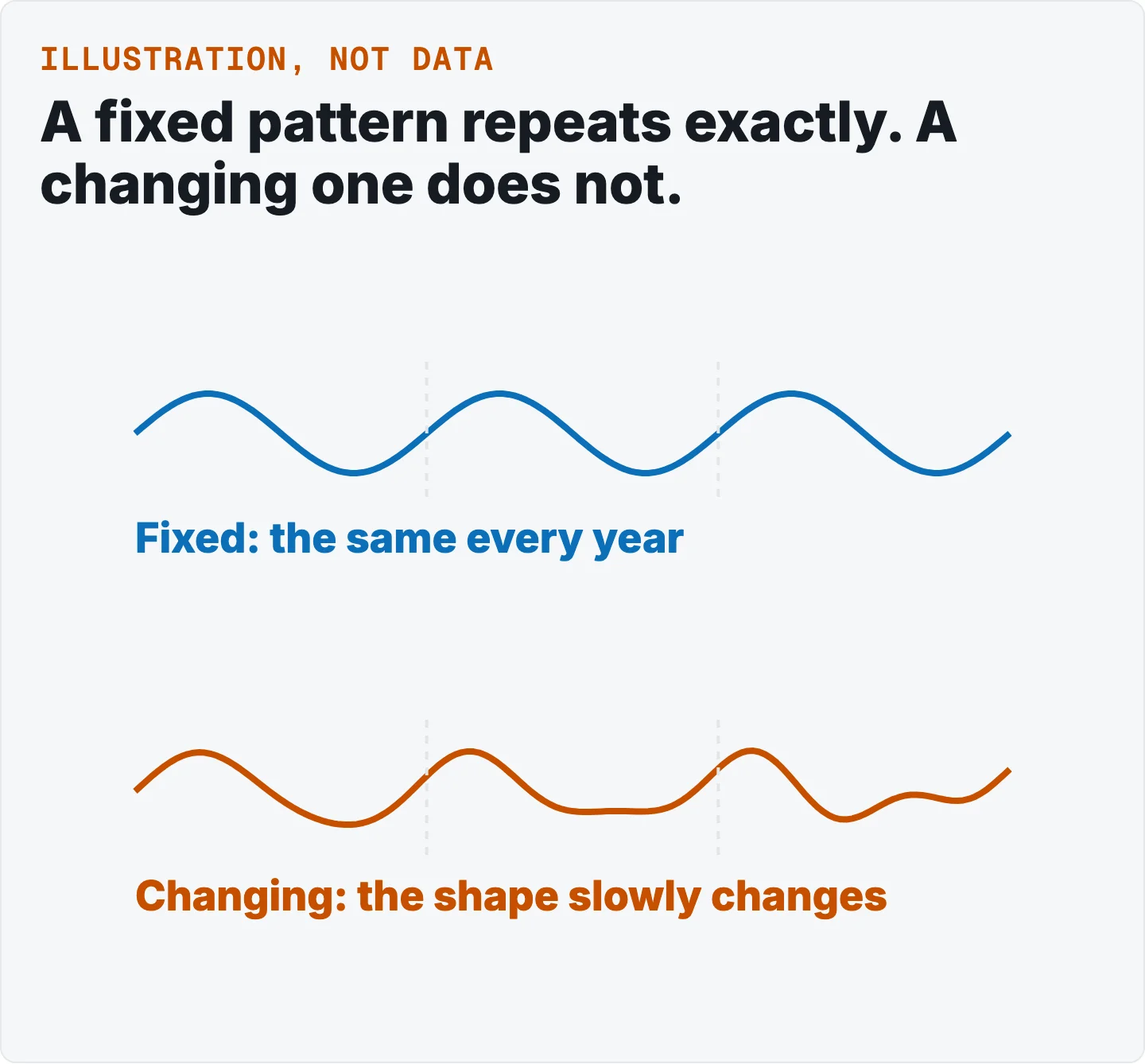
A periodic fit assumes the pattern never changes. Forcing an unchanging season shape is a choice, made by setting the window to infinity [3]. Our application. A pattern that is slowly drifting will be averaged flat under that choice.
The trend can hide a slow cycle. Because the trend line may contain cyclical swings [1], a slow cycle can sit in the trend and not show up as seasonal. Our example: a slow business cycle.
Gaps and outliers. One software example tells users to start by aggregating to monthly and filling any missing values [4]. R's default is to fail on missing values [5].
A short series. Our tool needs a minimum length, described below. We know of no published minimum.
How to run it on your own file
- Bring one date column and one number column, such as sales by month.
- Check you have enough history: just over two full cycles.
- Read the trend, the strength of the pattern, and the peak and trough seasons.
Run the free seasonality tool on your own monthly or weekly series (daily data gives a weekly cycle). For more, see our practical guide to seasonal decomposition.
What you need and what you get back
What your file needs: one date column and one number column, with just over two full cycles of data.
What you get back (these are facts about our tool, not general rules):
- It runs STL with a periodic season part, additive, with no log step and without the robust option. Our free tool is additive only.
- It infers the cadence from the median spacing of the dates. Daily data cycles weekly, weekly data cycles yearly, and monthly data cycles yearly. Other spacings are refused.
- It needs just over two full cycles of data. At least two cycle lengths plus one period. That is this tool's own rule. The sources we read state no minimum, so do not read it as a published law.
- Its strength is the formula above. The bands, weak below 0.3, moderate up to just under 0.6, and strong at 0.6 or more, are this tool's own choice and not from a source.
- It reports the peak and trough seasons as a percent above or below the trend (in the data's own units when the trend level is near zero).
How we checked it
Three things to know about how this page was written.
Every claim has a source or a label
Each statement is tagged to the numbered reference it came from, or marked as ours. Our own framing is not presented as a sourced rule.
Our tool is described as ours
What the free tool does is stated as facts about our tool, taken from its code. Its choices, such as its bands for how strong a pattern is, are its own.
No numbers from a dataset
This page uses no data, so it gives no benchmark, no typical seasonal swing and no forecast. The retail and carbon dioxide articles show the idea with numbers.
Questions people ask
What is seasonal decomposition?
Splitting a series into a trend, a season part and a rest [1][2].
Should I use an additive or multiplicative decomposition?
Look at whether the swings stay the same size as the level rises. If they do, additive. If they grow with the level, multiplicative [2].
What is STL, and why use it?
STL is a loess-based method. It handles any season period, lets the season part change over time, and can be made robust to outliers [3].
How do I measure how seasonal a series is?
With the strength formula, which is floored at 0 and is close to 1 when seasonality is strong [6]. The source gives no threshold for weak, moderate or strong. The 0.3 and 0.6 bands are our tool's own choice.
Is the seasonal part the same every year?
In STL it can change over time. A periodic setting holds it the same each year [3]. The classical method assumes it repeats from year to year [2].
References
- Decomposition of time series
- Hyndman, R. J. and Athanasopoulos, G. Forecasting: Principles and Practice (3rd ed.), Classical decomposition
- Hyndman, R. J. and Athanasopoulos, G. Forecasting: Principles and Practice (3rd ed.), STL decomposition
- statsmodels. STL
- R Documentation. stats::stl
- Hyndman, R. J. and Athanasopoulos, G. Forecasting: Principles and Practice (3rd ed.), Features based on STL