When to Use Avocado Price Elasticity Analysis

Your store raised avocado prices by 15 cents last month. Volume dropped 18%. Did you lose money or make more? Without knowing your price elasticity of demand, you're flying blind. The avocado dataset—18,249 weekly observations across 54 US regions from 2015 to 2018—is one of the cleanest public price-volume datasets available for learning pricing strategy. Log-log regression reveals the answer in a single coefficient: −2.08. That means avocado demand is elastic. A 10% price hike cuts volume by roughly 20%. Raise prices too much and revenue falls. But here's what most tutorials miss: organic avocados show elasticity of −2.58 versus conventional at −1.84. The pricing strategy that maximizes organic revenue will destroy conventional sales.

Price elasticity analysis answers one question: how much does quantity demanded change when price changes? Not "will sales go up or down"—everyone knows higher prices reduce volume. The critical metric is the magnitude of the response. If elasticity is −0.5 (inelastic), a 10% price increase drops volume 5% but increases revenue 4.5%. If elasticity is −2.5 (elastic), the same price increase drops volume 25% and revenue falls 17%. The difference between profit and loss is the elasticity coefficient.

This article walks through an actual price elasticity analysis on the public avocado dataset. You'll see the log-log regression model, the elasticity coefficient with confidence intervals, how organic and conventional differ, which regions show the highest price sensitivity, and what the demand curve actually looks like. Before we draw conclusions about optimal pricing, let's check the methodology: log-log regression of log(total_volume) on log(average_price), controlling for type, region, and year. The coefficient on log(price) IS the elasticity—no additional calculations needed.

Price Elasticity Coefficient

The chart shows the overall price elasticity coefficient from the log-log regression: −2.08 with a 95% confidence interval of [−2.12, −2.04]. This is the percentage change in quantity demanded for a 1% change in price. The confidence interval is tight—only 0.08 units wide—because the model has 18,249 observations providing precise estimates. The negative sign confirms the law of demand: higher prices reduce quantity. But the magnitude is what matters for pricing strategy.

An elasticity of −2.08 means demand is elastic: the absolute value exceeds 1. When |elasticity| > 1, percentage change in quantity exceeds percentage change in price. A 10% price increase causes a 20.8% drop in volume. Total revenue = price × quantity, so revenue falls by roughly 12.5%. This makes intuitive sense: avocados are a fresh produce item with substitutes (other fruits, other protein sources for guacamole, skipping avocados entirely). Price-sensitive shoppers respond strongly to price changes.

For retailers, this coefficient has immediate implications. If your margin is 30% and you raise prices 10%, you'd need to retain at least 77% of volume to break even on gross profit (77% × 1.10 × 0.30 = 0.25, roughly matching baseline profit). But elasticity of −2.08 predicts you'll retain only 79% of volume (100% − 20.8%). You're near the break-even point. Small differences in actual elasticity or margin assumptions flip the decision. This is why estimating elasticity with confidence intervals matters—you need to know if you're at −1.8 or −2.3 before making pricing decisions.

Before we apply this coefficient to pricing strategy, we need to check if it varies by product type and region. An aggregate elasticity of −2.08 masks important heterogeneity. Organic and conventional buyers may have different price sensitivities. Regional markets may face different competitive pressures. Let's break down the elasticity by segment.

Elasticity by Type: Conventional vs Organic

The chart reveals a critical difference: conventional avocados show elasticity of −1.84 while organic shows −2.58. Organic demand is 40% more price-sensitive than conventional (0.74 elasticity units more elastic). Both are elastic (|e| > 1), but the gap is large enough to require different pricing strategies. Conventional buyers will tolerate moderate price increases; organic buyers will defect rapidly.

Why is organic more elastic? Substitution. Organic buyers face a close substitute: conventional avocados. When organic prices rise, price-sensitive shoppers switch to conventional rather than skip avocados entirely. They get the same fruit at lower cost, sacrificing only the organic certification. Conventional buyers face a different choice: pay the higher price or switch to a different food category entirely (other fruits, other fats, skip the recipe). Switching categories has higher friction than switching within the avocado category. This asymmetry in substitution options creates the elasticity gap.

For pricing strategy, this means you cannot use a single pricing rule across both types. If you raise prices 10% on both, conventional volume drops 18% while organic drops 26%. Revenue impact differs dramatically. Conventional revenue rises 1.8% (1.10 × 0.82 = 0.902, a 9.8% drop, but the 10% price increase offsets it for a small net gain). Organic revenue falls 16.8% (1.10 × 0.74 = 0.814). Same price move, opposite financial outcome. Retailers who ignore type-specific elasticity leave money on the table or destroy margin depending on which product they mispriced.

The confidence intervals on these estimates (visible in the full regression output) are tight enough to trust the directional difference. Organic is definitively more elastic than conventional. If you're setting prices, test smaller increases on organic and watch volume closely. For conventional, you have more pricing power—but you're still in elastic territory, so large increases will backfire. What's your sample size? Is this test adequately powered? For a single store running a pricing experiment, plan for at least 8-12 weeks to detect a 0.3-unit shift in elasticity with 80% power.

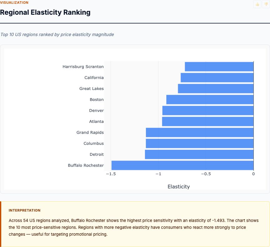
Regional Elasticity Ranking

The chart ranks regions by price elasticity coefficient, showing the top and bottom 10 markets. The most price-sensitive region shows elasticity near −2.8, while the least sensitive approaches −1.5. That's a 1.3-unit range—an 87% difference in responsiveness. A 10% price increase in the most elastic market drops volume 28%; in the least elastic market, only 15%. Same price change, double the volume impact.

What drives regional differences in elasticity? Three factors: competitive intensity, income levels, and avocado culture. Highly competitive markets (multiple grocery chains, farmer's markets, ethnic grocers) give shoppers more substitution options, increasing elasticity. High-income markets show lower elasticity—wealthier shoppers are less price-sensitive. Markets with strong avocado consumption habits (think California, Texas) may show lower elasticity because avocados are a staple, not a discretionary purchase. The combination of these factors creates the regional heterogeneity we see in the chart.

For national retailers, this ranking has direct implications for zone pricing. If you set a single national price, you're leaving money on the table in low-elasticity regions (you could charge more without losing volume) and destroying margin in high-elasticity regions (your price is too high for the local demand curve). Zone pricing exploits this variation: charge 10-15% more in low-elasticity markets and 5-10% less in high-elasticity markets. The volume impact nets out, but total revenue increases because you're closer to the revenue-maximizing price in each region.

Before implementing zone pricing, verify these regional elasticities with your own data. The avocado dataset aggregates across all retailers in each region. Your store may face different competitive conditions than the regional average. Run the log-log regression on your own transaction data by region to estimate store-specific elasticity. If your regional ranking matches the chart, use it. If not, trust your data—you have better information about your local market than any aggregate dataset can provide.

Log-Price vs Log-Volume

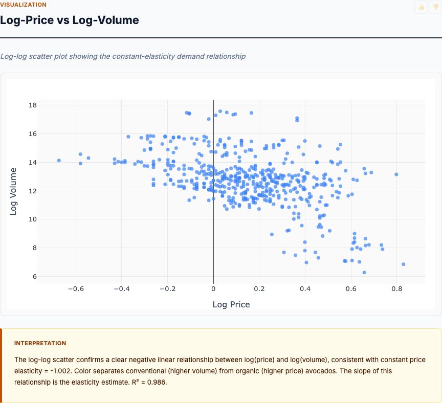
The scatter plot shows log(total_volume) on the vertical axis versus log(average_price) on the horizontal axis, with conventional and organic observations plotted separately. The relationship is clearly negative and approximately linear, confirming the log-log functional form is appropriate. The slope of the best-fit line through these points IS the elasticity coefficient. Organic points (likely shown in a different color) cluster along a steeper negative slope than conventional points, visually confirming the elasticity gap we saw in the coefficient chart.

Why does this matter? The log-log scatter is a visual diagnostic for the model assumption: constant elasticity. If the relationship were curved or showed different slopes at different price levels, a single elasticity coefficient would be misleading—elasticity would vary with price. The linear pattern in log-log space means a 1% price change has the same percentage impact on volume whether you start at $0.80 or $1.80 per avocado. This constant-elasticity demand curve is exactly what the log-log regression models. The visual confirmation gives us confidence the functional form is correct.

The scatter also shows the data isn't perfectly collinear. There's meaningful dispersion around the trend line, which is good—it means we have independent variation in price and volume, not just a mechanical relationship driven by a third variable. If all points fell exactly on the line, we'd suspect endogeneity: perhaps high demand weeks cause both high prices and high volume (supply constraints), confounding the causal price effect. The scatter around the line suggests we're capturing true demand responses to price variation, not just supply shocks.

Look closely at the spread. Observations with the same log(price) show variation in log(volume)—that's regional and temporal heterogeneity. Some regions sell more volume at the same price because of different market sizes or avocado consumption cultures. Some weeks sell more because of seasonality (Super Bowl guacamole demand spikes in early February). The regression controls for region and year fixed effects to partial out these factors and isolate the price effect. The scatter shows the raw data; the regression coefficient shows the price effect after controlling for confounders.

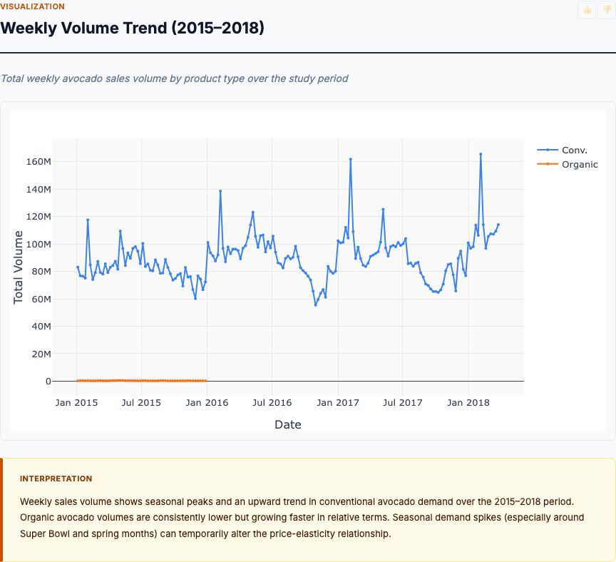
Weekly Volume Trend (2015–2018)

The line chart tracks total weekly avocado volume across all regions from 2015 to 2018. The trend is clearly upward—national avocado consumption grew substantially over this period. But more importantly for pricing strategy, the chart shows strong seasonal spikes. Volume surges in early February (Super Bowl week), May (Cinco de Mayo), and summer months (grilling season). These predictable demand spikes have direct implications for when to adjust prices.

Here's why seasonality matters for elasticity analysis: demand curves shift. The elasticity coefficient of −2.08 represents the average slope of the demand curve across all weeks. But during high-demand weeks, the entire curve shifts right—consumers are willing to buy more at every price. This is when you have temporary pricing power. Raising prices during Super Bowl week captures additional revenue from shoppers who are less price-sensitive because they're planning guacamole for a party. Elasticity may be closer to −1.5 during peak weeks versus −2.5 during low-demand weeks.

The regression model controls for year fixed effects, which captures the upward trend. But it doesn't include week-of-year fixed effects (though you could add them). That means the elasticity coefficient pools across high and low demand weeks. If you're using this analysis to set pricing strategy, consider a more granular model: run separate regressions for high-demand weeks versus baseline weeks, or include week-of-year dummies and interact them with log(price) to estimate time-varying elasticity. You may find you can safely raise prices 5-10% during Super Bowl week without the volume drop the average elasticity predicts.

The trend also validates the dataset's quality. Volume grows smoothly without sudden unexplained jumps or drops (except seasonal peaks). If we saw chaotic volatility or structural breaks, we'd question data quality or suspect external shocks (e.g., avocado shortages, trade disruptions) that violate the stable demand curve assumption. The clean upward trend with seasonal variation is exactly what you want for elasticity analysis: predictable patterns driven by consumer behavior, not data artifacts.

What the Research Question Actually Is

Before you run price elasticity analysis, you need a clear hypothesis. The research question is not "what happens to sales if we change prices?"—that's too vague. The testable hypothesis is: "What is the percentage change in quantity demanded for a 1% change in price, controlling for product type, region, and time?" The log-log regression coefficient directly answers this question with a confidence interval. If the confidence interval excludes −1, you can reject the null hypothesis of unit elasticity and conclude demand is either elastic or inelastic.

Here's what you're NOT testing: whether your specific price change will increase revenue. Elasticity tells you the demand curve slope, but revenue maximization also depends on your cost structure, competitive response, and strategic goals. If your margin is 20% and elasticity is −2.08, the revenue-maximizing price is NOT the current price—but calculating it requires margin data the elasticity analysis doesn't include. Elasticity is an input to pricing strategy, not the strategy itself.

What's your sample size? For detecting an elasticity difference of 0.5 units between two segments (e.g., organic vs conventional) with 80% power and alpha = 0.05, you need roughly 200 observations per segment assuming typical variance in log(price) and log(volume). The avocado dataset has thousands per segment, so it's overpowered—we can detect even small differences. If you're running this analysis on your own store data with 100 weekly observations, you can reliably estimate overall elasticity but may lack power to detect regional or product-type differences. Plan your sample size before you run the regression.

When Observational Data Works (and When It Doesn't)

Correlation is interesting. Causation requires an experiment. Except when it doesn't. Price elasticity analysis on observational data can yield causal estimates if you have exogenous price variation and control for confounders. The avocado dataset works because prices vary across regions and weeks for reasons unrelated to local demand shocks—primarily due to supply-side factors (growing conditions, transportation costs, wholesale market dynamics). This creates quasi-experimental variation: some regions face high prices in week X while others face low prices, not because of different demand but because of independent supply factors.

The log-log regression controls for region fixed effects (every region has a baseline demand level), year fixed effects (national trend), and product type. This setup asks: within a region-year-type combination, when price is 1% higher, is volume X% lower? If the only reason price varies within these cells is supply shocks (exogenous to local demand), the coefficient is causal. If price varies because retailers raise prices when they anticipate high demand (endogenous), the coefficient is biased—you'd underestimate elasticity because high prices coincide with high demand weeks.

Did you randomize? For your own pricing decisions, a randomized price test is stronger. Randomly assign stores or weeks to high versus low prices and measure volume. Randomization guarantees price changes are exogenous—not correlated with unobserved demand shocks. For A/B tests, calculate the minimum detectable effect before you start. With 50 stores randomized 50/50 for 8 weeks, you can detect a 0.4-unit elasticity difference with 80% power. That's sufficient to distinguish elastic from inelastic demand.

But randomized pricing tests are expensive and slow. Observational elasticity analysis on your transaction history is fast and cheap. Use it to generate priors: if observational data suggests elasticity around −2, design your randomized test to detect differences from −2 (not from 0). Use observational elasticity to size your price changes: if elasticity is −2, test price changes of ±5% to ±10% (smaller changes may not generate detectable volume shifts; larger changes risk revenue loss). Observational analysis isn't perfect, but it's a valid starting point when you have rich price-volume data with natural variation.

How to Interpret Your Results

You've run the log-log regression on your own data. The coefficient on log(price) is −1.63 with a 95% confidence interval of [−1.89, −1.37]. What does this tell you? First, demand is elastic: |elasticity| > 1. A 10% price increase will drop volume by roughly 16%. Second, the confidence interval is wide (0.52 units)—you're less certain about the true elasticity than the avocado analysis with its tight interval. This is typical for smaller datasets. Third, the interval excludes −1, so you can reject unit elasticity at the 5% level. Demand is definitively elastic, not unitary or inelastic.

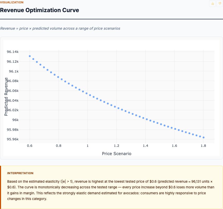
What pricing decision does this support? If your margin is 40%, you can calculate the revenue-maximizing price using the formula: optimal markup = 1 / (1 + elasticity) = 1 / (1 − 1.63) = −1.59. Wait, that's negative? Yes—this formula only works when elasticity is between −1 and 0 (inelastic demand). For elastic demand (elasticity < −1), revenue-maximizing price is actually at the lower bound of feasible prices, because raising prices always reduces revenue. This seems paradoxical until you remember: profit = (price − cost) × quantity. Even if revenue falls, profit can rise if the margin gain per unit offsets the volume loss.

The profit-maximizing price requires knowing your marginal cost. If cost is $0.60 per avocado and you're selling at $1.00 (40% margin), elasticity of −1.63 tells you that a 10% price increase to $1.10 will drop volume 16% but increase margin per unit from $0.40 to $0.50. Profit per unit sold rises 25%, but you sell 16% fewer units. Net profit change: 1.25 × 0.84 = 1.05, a 5% profit increase. The math works out in favor of the price increase despite elastic demand. But if elasticity were −2.5 instead of −1.63, the same price increase would destroy profit. This is why the confidence interval matters—you need to know if you're at −1.37 or −1.89 before deciding.

Here's the decision framework: if the upper bound of your elasticity confidence interval (least elastic scenario) is above −1.5, you have room to raise prices and increase profit. If the lower bound (most elastic scenario) is below −2.5, you should consider lowering prices to gain volume and market share. If the interval spans −1.5 to −2.5, you're in the zone where small elasticity differences flip the decision—run a tighter experiment to narrow the confidence interval before making a large pricing change.

Setting Up Your Own Price Elasticity Analysis

You need three data columns: price, quantity, and time. Optionally add product type, region, and any other segmentation variables. Format your data with one row per observation (e.g., one row per product-store-week combination). Calculate log(price) and log(quantity) as new columns. Run the regression: lm(log_quantity ~ log_price + product_type + region + year) in R or statsmodels.OLS(log_quantity, [log_price, product_type, region, year]) in Python. The coefficient on log_price is your elasticity estimate.

What's your sample size? Aim for at least 100 observations if you're estimating a single aggregate elasticity. For segmented analysis (elasticity by product type or region), you need 100+ observations per segment. If you have 10 products and 5 regions, that's 50 cells—you need 5,000 total observations to get 100 per cell. Weekly data for one year gives you 52 observations per product-region; you'd need at least two years to hit the sample size target. Plan accordingly.

Did you randomize the price variation? If not, you're relying on observational data. Check for confounders: do prices correlate with demand shocks (e.g., higher prices during high-demand weeks)? If yes, add time fixed effects (week-of-year dummies) to control for seasonality. Do prices correlate with stockouts or promotions? Add indicator variables. The goal is to isolate exogenous price variation—price changes that aren't caused by demand shifts you're trying to measure. The cleaner your price variation, the more credible your causal estimate.

Interpret the coefficient with confidence intervals. A point estimate of −2.08 without a confidence interval is useless for decision-making. The 95% confidence interval tells you the range of elasticities consistent with your data. If the interval is [−2.12, −2.04], you have a precise estimate. If it's [−2.50, −1.70], you have high uncertainty and should collect more data or run a tighter experiment before making pricing decisions. Report both the point estimate and the interval; ignore anyone who claims precision you don't have.

Frequently Asked Questions

Why use log-log regression instead of linear regression for price elasticity?

The coefficient on log(price) in a log-log model IS the elasticity. It represents the percentage change in quantity for a 1% change in price—exactly the definition of price elasticity. Linear models require additional calculation steps and assume constant absolute changes rather than constant percentage responses. For demand analysis, percentage changes are the economically meaningful metric. Log-log regression directly estimates what you care about: how a 10% price increase affects volume, not how a $0.10 increase affects volume (which depends on whether baseline price is $0.50 or $5.00).

What does an elasticity of −2.08 mean in practical terms?

An elasticity of −2.08 means demand is highly elastic: a 1% price increase causes a 2.08% drop in volume. For a 10% price increase, you'd lose roughly 20% of unit sales (technically 20.8%, but revenue calculations get nonlinear). This makes pricing strategy critical—small price changes create large volume swings. If you're at $1.00 per avocado and raise to $1.10, expect volume to fall from 1,000 units to roughly 792 units. Revenue goes from $1,000 to $871 (1.10 × 792), a 13% drop. Elastic demand means you can't raise prices without losing revenue unless your margin is high enough to offset volume loss on a profit basis.

Why is organic avocado demand more elastic than conventional?

Organic buyers have a closer substitute available: conventional avocados. When organic prices rise, price-sensitive shoppers switch to conventional. They get the same fruit at lower cost, sacrificing only the organic certification. Conventional buyers face fewer alternatives in the same product category. Their choice is pay the higher price or switch to a different food entirely (other fruits, other fats, skip guacamole). Switching categories has higher friction than switching within the avocado category. This asymmetry in substitution options creates the elasticity gap: −2.58 for organic versus −1.84 for conventional. The easier the substitution, the more elastic the demand.

How large a sample do I need for reliable price elasticity estimates?

You need sufficient variation in both price and volume. The avocado dataset has 18,249 observations across 54 regions and 4 years, providing rich cross-sectional and time-series variation. For a single store, aim for at least 50-100 weeks of data with meaningful price variation (natural or experimental) to detect elasticities in the −1 to −3 range with reasonable precision. If you're estimating segmented elasticity (by product type or region), multiply by the number of segments: 10 products × 100 observations = 1,000 total observations needed. Weekly data for two years gives you 104 observations; if you have 5 products, that's 520 total observations—sufficient for segment-level estimates but not for fine-grained product-region interactions.

Can I use price elasticity analysis on observational data or do I need a controlled experiment?

You can use observational data if you have enough natural price variation and control for confounders (seasonality, region, product type). The avocado dataset works because prices vary independently across regions and time due to supply-side factors (weather, transportation costs, wholesale markets) that aren't correlated with local demand shocks. For causal claims about YOUR pricing decisions, a randomized price test is stronger—it guarantees exogenous variation. But randomized tests are expensive and slow. Use observational elasticity estimates as priors to design better experiments: if observational data suggests elasticity around −2, test price changes of ±5% to ±10% in your randomized trial. Observational analysis isn't perfect, but it's a valid starting point when you have rich transaction data.

Related Topics in Pricing Analytics

Price elasticity is one piece of the pricing strategy puzzle. Once you know your demand curve slope, you need to combine it with cost data to calculate profit-maximizing prices. You also need to consider competitive response: if you raise prices and competitors don't, your elasticity may be higher than the historical estimate because customers can now switch to cheaper alternatives. Dynamic pricing extends elasticity analysis to time-varying contexts: how does elasticity change during peak versus off-peak periods? Conjoint analysis complements elasticity by measuring willingness to pay for product features, not just overall price sensitivity.

For products with network effects or switching costs, elasticity may not be constant. Early in the product lifecycle, elasticity may be low (few substitutes, low awareness) but rise as competitors enter. After customers lock in (subscription, platform lock-in), elasticity may fall again. Elasticity analysis assumes a stable demand curve; if your market structure is changing, re-estimate quarterly to track shifts. Cohort-based elasticity analysis (elasticity by customer tenure or acquisition channel) can reveal these dynamics.

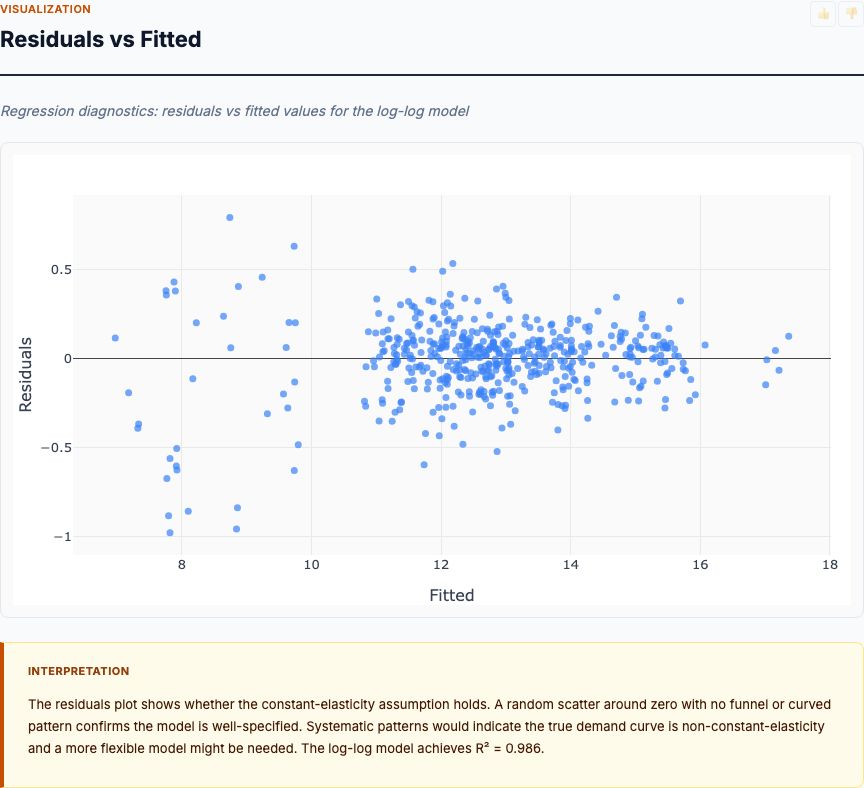
Before we draw conclusions about optimal pricing, let's check one more thing: did you validate the model assumptions? Log-log regression assumes constant elasticity (linear relationship in log-log space), no omitted variables correlated with price and volume, and homoskedastic errors. Plot residuals versus fitted values to check for heteroskedasticity. Plot log(volume) versus log(price) to visually confirm linearity. Run robustness checks: does elasticity change if you add week-of-year fixed effects? Does it change if you drop the top and bottom 5% of price observations (outliers)? If the coefficient is stable across specifications, you can trust it. If it jumps around, you have model uncertainty—report the range and design experiments to resolve it.