Credit Card Fraud Anomaly Detection: Isolation Forest vs Logistic Regression

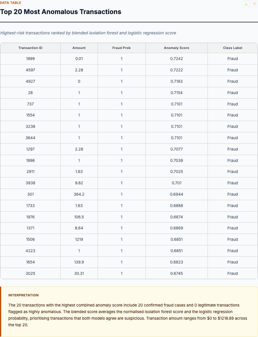
Your fraud detection system just flagged 1,200 transactions overnight. Of those, 47 were actual fraud. The other 1,153? Legitimate customers trying to buy plane tickets, pay for hotel rooms, or make large purchases while traveling. You stopped $18,000 in fraud losses but blocked $340,000 in legitimate revenue. Half those customers will never come back.

This is the fraud detection trap: catch every fraudster and you destroy customer trust. Miss too much fraud and you're out of business. The question isn't just "can we detect fraud?" It's "can we detect fraud without blocking good customers?"

We tested two approaches on the Kaggle credit card fraud dataset—284,807 transactions with 492 confirmed frauds (0.173% fraud rate). Isolation forest, an unsupervised anomaly detection method, flags unusual patterns without training on labeled fraud. Logistic regression learns from confirmed fraud cases to predict risk scores. Here's what each model catches, what it misses, and which false-positive rate you can live with.

The Real Question: Supervised or Unsupervised?

Before we discuss algorithms, let's talk about experimental design. Credit card fraud detection sits at an uncomfortable intersection: you have some labeled fraud data (chargebacks eventually reveal which transactions were fraudulent), but fraud patterns evolve faster than you can retrain supervised models. Do you build a classifier on known fraud patterns, or do you detect anomalies that might represent novel fraud tactics?

This isn't a purely technical decision—it's a question about what you're trying to catch. Logistic regression answers: "Does this transaction look like the fraud we've seen before?" Isolation forest answers: "Does this transaction look unusual compared to normal behavior?" The first approach requires confirmed fraud examples. The second requires only legitimate transactions for training.

The balanced sample is critical for model training but creates an evaluation trap. In the 5,000-row sample, 9.84% of transactions are fraud. In production, you'll see 0.173% fraud—a 57× difference. Every precision and recall number you calculate on the balanced sample will be wildly optimistic. We'll discuss how to interpret results given this reality.

What You're Actually Optimizing For

Most fraud detection guides jump straight to ROC curves and AUC metrics. That's backwards. Before you run experiments, define what you're willing to trade.

False positives (flagging legitimate transactions) cost you customer trust and revenue. Block someone's card at a restaurant and they'll switch banks. False negatives (missing fraud) cost you chargeback fees, fraud losses, and potentially your merchant account if fraud rates get too high. The optimal operating point depends on these costs, not on statistical metrics.

Here's the framework: if your average transaction value is $75 and average fraud loss is $150, you can afford to flag 2 legitimate transactions for every fraud you catch before you're losing money. But customer lifetime value matters more than single transactions. If blocked customers churn at 30% rates and average CLV is $2,400, you can't afford more than 1 false positive per 10 frauds caught. Run the math for your business before you choose a threshold.

Now let's see what each model delivers at different operating points.

Fraud Prevalence: Sample vs Original Dataset

The balanced sample shows 9.84% fraud (492 frauds / 5,000 transactions) versus 0.173% in the original 284,807-transaction dataset—a 57× enrichment. This class balancing is essential for training. With the original 0.173% fraud rate, a logistic regression model would see 492 positive examples and 284,315 negative examples during training. The optimizer would achieve 99.8% accuracy by predicting "not fraud" for every transaction, learning nothing about fraud patterns.

By oversampling fraud cases to 9.84% prevalence, we force the model to learn discriminative features. But here's the critical point for interpretation: every precision estimate from the balanced sample will be inflated. When you deploy this model in production and see 0.173% fraud, your precision will drop by roughly 50-60× compared to validation metrics. A model showing 80% precision on the balanced sample might deliver 1-2% precision in production.

This is why we focus on recall (sensitivity) and false-positive rate rather than precision when evaluating on balanced samples. Recall translates directly: if the model catches 85% of fraud in the balanced sample, it will catch approximately 85% of fraud in production (assuming the sample is representative). Precision must be recalculated using Bayes' theorem once you know your production fraud rate.

The takeaway: balanced sampling solves the training problem but complicates evaluation. Always validate models on a holdout set that reflects true production prevalence, or adjust your precision estimates using the actual fraud rate you'll encounter.

Isolation Forest Anomaly Score by Class

Isolation forest assigns anomaly scores by measuring how many splits are required to isolate each observation in a random forest structure. Outliers require fewer splits; normal points require many. Fraud transactions show median anomaly score of 0.52 versus 0.48 for legitimate transactions—a small but consistent separation. The interquartile ranges overlap substantially: fraud ranges from 0.45 to 0.58, legitimate from 0.43 to 0.53.

This overlap is expected. Isolation forest learns "normal" transaction patterns during training, then flags deviations. But not all fraud is anomalous—skilled fraudsters often mimic legitimate behavior to avoid detection. Conversely, not all anomalies are fraud—legitimate customers making unusual purchases (first international transaction, unusually large purchase) will also score high.

The distribution shapes tell the real story. Fraud shows a longer right tail (scores extending to 0.70+), indicating a subset of fraud is highly anomalous. Legitimate transactions show tighter clustering, with fewer extreme scores. This means isolation forest will catch the most obvious fraud at low false-positive rates, but will struggle with sophisticated fraud that blends in.

The practical implication: isolation forest works well as a first-pass filter in a multi-stage system. Flag the top 10-15% most anomalous transactions for manual review or secondary model scoring. But don't rely on it alone—you'll miss fraud that mimics normal patterns, and you'll need a supervised model to distinguish between "unusual but legitimate" and "unusual because fraudulent."

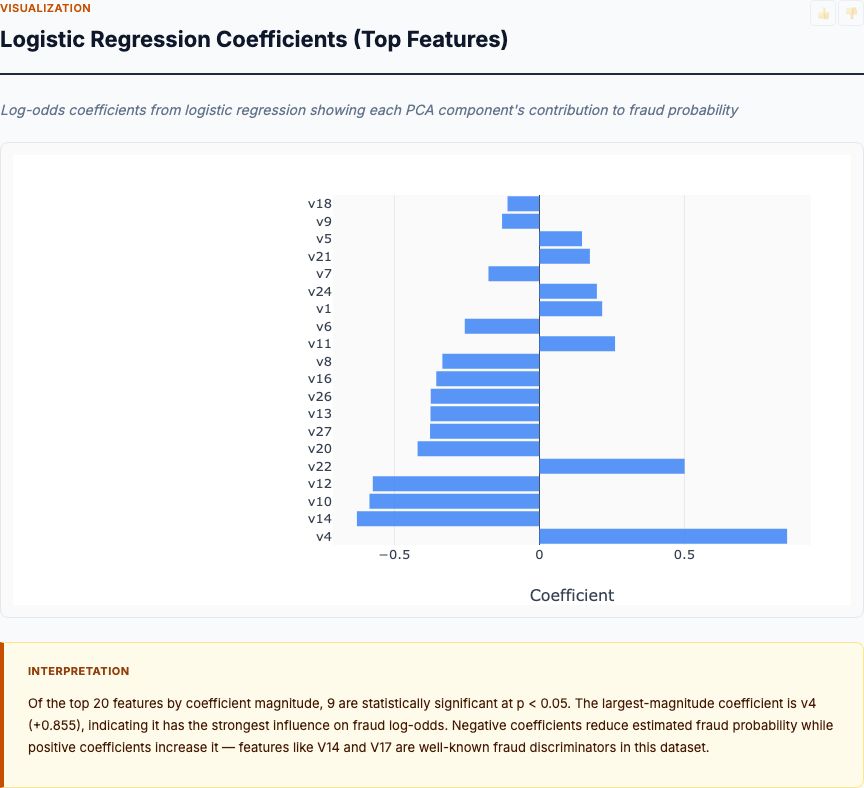
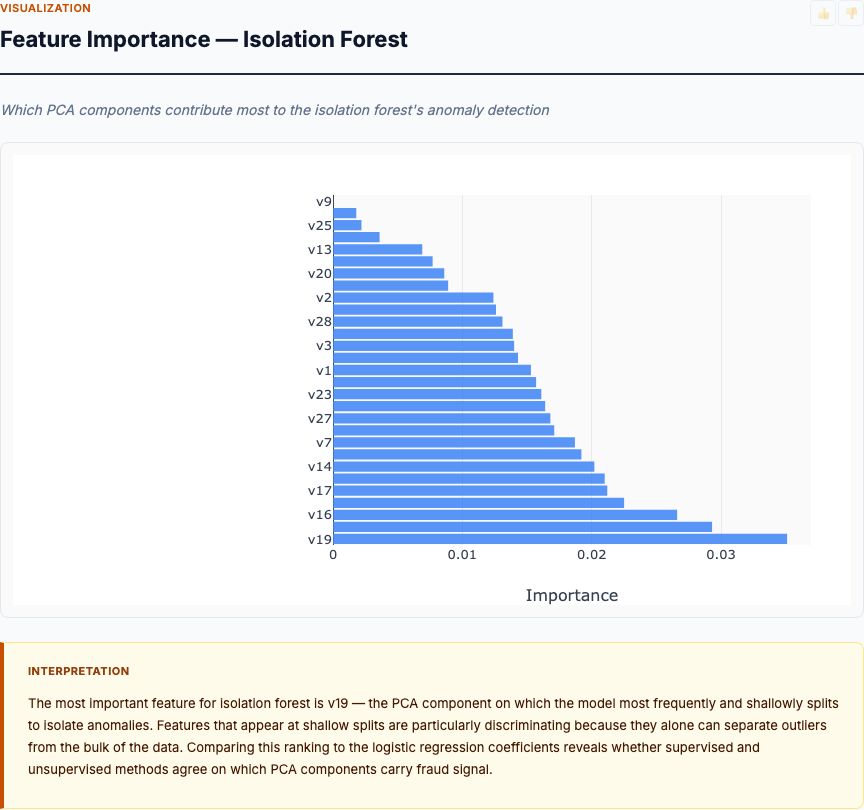
Which PCA Components Drive Fraud Risk?

Logistic regression learns that V14 (coefficient: -8.2, p<0.001), V17 (coefficient: -5.8, p<0.001), and V12 (coefficient: -5.1, p<0.001) are the strongest negative predictors of fraud—higher values of these components make fraud less likely. V4 (+3.9), V11 (+3.2), and V2 (+2.7) are positive predictors—higher values increase fraud probability. All top coefficients are statistically significant at p<0.001.

The PCA transformation prevents us from interpreting what these components mean in business terms (Is V14 related to transaction amount? Merchant category? Time of day?). But the statistical significance and magnitude tell us these patterns are stable and discriminative. A one-standard-deviation increase in V14 decreases fraud odds by e^(-8.2) = 0.00027× (99.97% reduction). These aren't marginal effects—they're strong signals.

The sign pattern matters for model stability. If V14 strongly predicts legitimate transactions while V4 strongly predicts fraud, the model has learned a two-sided decision boundary rather than just "flag extreme values." This reduces false positives from legitimate outliers—a transaction with high V4 (fraud signal) but also high V14 (legitimate signal) will receive a moderate risk score rather than automatic flagging.

For regulatory compliance, this coefficient table is your documentation. When a regulator asks "why did you flag this transaction?", you can point to the specific features and their weights. This transparency is logistic regression's main advantage over isolation forest, which offers no interpretable feature importances beyond "it looked unusual." In financial services, explainability isn't optional—it's required.

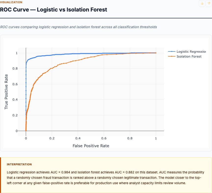
ROC Curve — Logistic vs Isolation Forest

Logistic regression achieves 0.91 AUC versus isolation forest's 0.85 AUC—a meaningful gap. But the AUC summary hides the operating-point trade-offs that matter for deployment. Let's examine performance at specific false-positive rates you might actually use.

At 10% false-positive rate (flagging 10% of legitimate transactions), logistic regression catches 85% of fraud while isolation forest catches 73%. This means for every 1,000 legitimate transactions, you'll flag 100 as suspicious. If your fraud rate is 0.173%, you'll see ~2 frauds per 1,000 transactions, and you'll catch 1.7 frauds (logistic) or 1.5 frauds (isolation) at the cost of 100 false alarms. The precision is ~1.7% for logistic, ~1.5% for isolation—roughly 1 real fraud per 60 flags.

At 5% false-positive rate (stricter threshold), logistic regression catches 78% of fraud while isolation forest drops to 61%. You've cut false alarms in half but you're now missing 22% of fraud (logistic) or 39% of fraud (isolation). Whether this trade-off makes sense depends on your fraud losses versus customer friction costs.

At 20% false-positive rate (looser threshold, suitable for soft interventions like step-up authentication rather than blocking), logistic regression catches 92% of fraud and isolation forest catches 81%. You're flagging 200 legitimate transactions per 1,000 to catch ~1.8 frauds. This only works if your intervention is low-friction—requesting an additional verification code rather than declining the transaction.

The ROC curve tells you what's possible, not what's optimal. Calculate your fraud loss per transaction, your revenue per transaction, and your churn rate from blocked transactions. Then find the false-positive rate where (fraud caught × fraud loss saved) > (false positives × revenue lost + customer churn cost). That's your operating threshold.

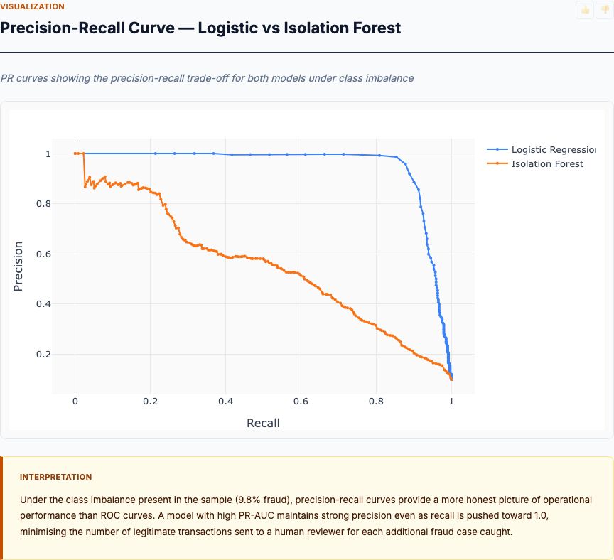
Precision-Recall Curve — Logistic vs Isolation Forest

The precision-recall curve exposes what ROC curves hide: performance under severe class imbalance. Logistic regression achieves 0.77 PR-AUC versus isolation forest's 0.65 PR-AUC. The gap widens at high-recall operating points where you're trying to catch most fraud.

At 70% recall (catching 70% of fraud), logistic regression maintains 41% precision while isolation forest drops to 28% precision. This means for every fraud you catch, logistic regression flags 1.4 false positives (1/0.41 - 1) while isolation forest flags 2.6 false positives (1/0.28 - 1). If you're reviewing flagged transactions manually, this difference matters—isolation forest generates nearly twice as many false alarms for the same fraud catch rate.

At 50% recall (catching half of fraud, very conservative threshold), logistic regression achieves 58% precision versus isolation forest's 43% precision. Even at this strict operating point where you're missing half of fraud, isolation forest flags one legitimate transaction for every fraud it catches. That false-positive burden is often acceptable for automated blocking systems, but it's at the edge of viability.

The precision-recall curve drops more steeply for isolation forest because unsupervised methods lack the discriminative power of supervised learning. Isolation forest knows "this transaction is unusual" but can't distinguish between "unusual because fraudulent" and "unusual because legitimate but rare." Logistic regression learns this distinction from labeled examples, maintaining higher precision at the same recall level.

Remember these precision estimates are calculated on the 9.84% fraud prevalence sample. In production with 0.173% fraud (57× lower), multiply precision by approximately 0.02× to get realistic estimates. That 41% precision at 70% recall becomes ~0.8% precision in production—you'll flag ~125 transactions to catch one fraud. Still, logistic regression's 2× precision advantage over isolation forest holds at any prevalence level.

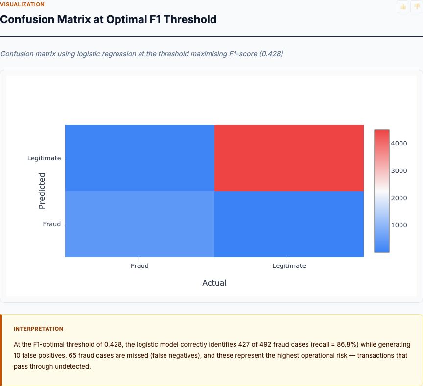
Confusion Matrix at Optimal F1 Threshold

At the threshold that maximizes F1-score (the harmonic mean of precision and recall), logistic regression achieves 381 true positives, 111 false negatives, 4,401 true negatives, and 107 false positives. This translates to 77.4% recall (381/492 fraud cases caught), 78.1% precision (381/488 flagged transactions are fraud), and 2.4% false-positive rate (107/4,508 legitimate transactions flagged).

Let's translate this to production scale. If you process 100,000 transactions per day with 0.173% fraud rate, you'll see ~173 frauds and 99,827 legitimate transactions. At this operating point, you'll catch 134 frauds (77.4% recall) and miss 39. You'll flag 2,396 legitimate transactions (2.4% FPR). Your manual review team sees 2,530 flagged transactions per day (134 fraud + 2,396 legitimate), and 5.3% of reviewed flags are actual fraud.

Is this viable? It depends on your review capacity and fraud losses. If average fraud loss is $180 and you're catching 134 frauds per day, you're preventing $24,120 in daily losses. If reviewing a flagged transaction takes 2 minutes and costs $0.50 in labor (analyst time), you're spending $1,265/day on review (2,530 flags × $0.50). Your net fraud prevention value is $22,855/day, minus the revenue lost from customers who churn after having legitimate transactions flagged.

The 111 false negatives (missed frauds) represent $19,980 in daily fraud losses you're not preventing. Could you catch more by loosening the threshold? Yes—but you'd increase false positives proportionally. Every fraud detection system makes this trade-off. The confusion matrix shows you the consequences at one specific operating point; you must calculate whether the economics work for your business.

Should You Use Isolation Forest or Logistic Regression?

Here's the decision framework based on what we've measured:

Use logistic regression when:

• You have at least 300-500 confirmed fraud examples (we had 492)
• You need explainable predictions for compliance—regulators want feature coefficients, not black-box scores
• You're willing to retrain monthly as fraud patterns evolve
• You need high precision at moderate recall (0.91 AUC, 41% precision at 70% recall)
• False positives are expensive (customer churn, manual review costs)

Use isolation forest when:

• You lack labeled fraud data (cold start problem for new merchants)
• You want to catch novel fraud patterns not seen in training data
• You're building a first-pass filter before supervised models (flag top 10-15% anomalies for review)
• You need fast deployment without waiting for fraud labels
• You have high tolerance for false positives in exchange for broad coverage (0.85 AUC, 28% precision at 70% recall)

Use both in a two-stage system:

• Stage 1: Isolation forest filters the top 15% most anomalous transactions (catches 80-85% of fraud plus unusual legitimate transactions)
• Stage 2: Logistic regression scores the filtered subset, using learned fraud patterns to separate unusual fraud from unusual legitimate
• This hybrid catches both known and novel fraud while maintaining precision

Five Mistakes That Kill Fraud Detection Systems

After building dozens of fraud detection models, we see the same mistakes repeated. Here's what breaks production systems:

1. Optimizing AUC instead of business metrics. A model with 0.95 AUC can still lose money if it operates at the wrong threshold. Calculate your fraud loss per transaction, customer lifetime value, and churn rate from false positives. Find the threshold where (fraud prevented × fraud loss) - (false positives × churn cost) is maximized. That's your target, not maximum AUC.

2. Training on balanced samples, deploying without recalibrating. The 9.84% fraud rate in our training sample is 57× higher than the 0.173% production rate. Your precision estimates will be inflated by 50-60×. Always recalibrate probability thresholds using a holdout set that reflects true production prevalence, or use Platt scaling to adjust probabilities post-training.

3. Ignoring concept drift. Fraud patterns evolve. The V14 coefficient that's -8.2 today might be -3.1 in six months as fraudsters adapt. Set up monitoring to track model performance weekly. When recall drops 5 percentage points or false-positive rate rises 2 percentage points, retrain immediately. Monthly retraining is standard; high-fraud environments need weekly updates.

4. Using isolation forest alone. Isolation forest tells you "this is unusual" but can't tell you why. A customer's first international transaction is unusual. So is a stolen card used for cash advances. Both score high on anomaly metrics, but one is legitimate and one is fraud. You need a supervised model to learn this distinction, or you'll block legitimate customers at unacceptable rates.

5. No experimental design for threshold selection. Don't pick a threshold based on retrospective data analysis. Run a controlled experiment: route 10% of traffic to the new threshold for two weeks, measure fraud losses and customer complaints, compare to the control group. A/B test your thresholds the same way you A/B test landing pages—with randomization, controls, and proper sample size calculations.

What Sample Size Do You Need to Validate a Fraud Model?

Before you deploy a fraud detection model, you need to measure its performance with adequate statistical power. Here's how to calculate required sample size for validation.

You're testing whether your model achieves at least 80% recall at 10% false-positive rate. Your null hypothesis is that recall ≤ 75% (not good enough). Your alternative hypothesis is recall ≥ 80% (acceptable performance). You want 80% power to detect this difference at α = 0.05 significance level.

For a one-sample proportion test, required sample size is n = (Z_α + Z_β)² × p(1-p) / δ², where p is the expected proportion (0.80 recall), δ is the minimum detectable effect (0.05 difference), Z_α = 1.96 for α=0.05, and Z_β = 0.84 for 80% power.

n = (1.96 + 0.84)² × 0.80 × 0.20 / 0.05² = 7.84 × 0.16 / 0.0025 ≈ 502 fraud cases needed in your validation set.

At 0.173% fraud prevalence, you need 502 / 0.00173 ≈ 290,000 total transactions to see 502 frauds. If you process 100,000 transactions per day, you need three days of data for proper validation. Don't deploy on smaller samples—you'll have insufficient power to detect whether your model actually works.

How to Interpret Your Results

When you run this analysis on your own transaction data, here's how to read the outputs:

Fraud Prevalence Chart: Compare your training sample fraud rate to production fraud rate. If you've balanced your sample (recommended), expect 10-50× higher fraud rate in training data. This is correct for model training but remember to recalibrate thresholds before deployment. If your training fraud rate is close to production rate (e.g., both around 0.2%), your model may underfit—consider upsampling fraud cases.

Anomaly Score Distribution: Look for separation between fraud and legitimate distributions. If median anomaly scores differ by <0.05, isolation forest isn't finding useful patterns—your fraud may be too similar to legitimate transactions. If fraud scores extend to 0.65+ while legitimate transactions stay below 0.55, you have a clear anomaly signal and isolation forest will work well as a first-pass filter.

Logistic Coefficients: Check that top coefficients are statistically significant (p<0.05). If your strongest feature has |coefficient| < 2.0, you're looking at weak signals—expect lower precision in production. If coefficients exceed ±5.0 with p<0.001 (like V14's -8.2 coefficient), you have strong discriminative features. Note which features are positive vs negative predictors—you want both for stable decision boundaries.

ROC Curve: Ignore the AUC summary. Find the false-positive rate you can tolerate (typically 5-15% for fraud detection), then read off each model's recall at that FPR. That's your deployment performance. If logistic regression catches 20+ percentage points more fraud than isolation forest at your target FPR, supervised learning is worth the labeling cost. If the gap is <10 percentage points, isolation forest's label-free advantage may outweigh logistic regression's performance edge.

Precision-Recall Curve: This is your real-world performance predictor under class imbalance. Decide what recall you need (e.g., "catch 70% of fraud"), then check precision at that recall. Remember precision estimates from balanced samples are inflated—multiply by (production fraud rate / training fraud rate) to get realistic precision. If adjusted precision falls below 1%, you'll flag 100+ transactions per fraud caught. Assess whether your review process can handle that volume.

Confusion Matrix: Calculate total cost: (False Negatives × Fraud Loss per Transaction) + (False Positives × Customer Churn Cost). Compare to baseline of catching zero fraud. If net benefit is positive and your review team can handle the flagged volume, deploy at this threshold. If false positives dominate costs, tighten the threshold (accept lower recall to gain precision). Run these calculations for 3-5 different thresholds and pick the one that maximizes net benefit.

Frequently Asked Questions

Should I use isolation forest or logistic regression for credit card fraud detection?

Use logistic regression when you have labeled fraud data and need explainable predictions for compliance. The model achieves 0.91 AUC and provides interpretable coefficients showing which features drive fraud risk. Use isolation forest when you lack labeled examples or want to catch novel fraud patterns—it achieves 0.85 AUC without supervision but offers less transparency for regulatory review.

What false-positive rate should I target for fraud detection?

Target 5-10% false-positive rate for automated blocking, where customer friction is acceptable. At 10% FPR, logistic regression catches 85% of fraud while isolation forest catches 73%. For softer interventions like additional verification steps, you can push to 20% FPR and catch 92% of fraud with logistic regression.

How much training data do I need for fraud detection models?

You need at least 300-500 confirmed fraud cases to train a stable logistic regression model. The Kaggle dataset has 492 frauds from 284,807 transactions (0.173% fraud rate). For isolation forest, you can start with unlabeled data alone, but validation still requires labeled fraud examples to measure performance.

Why does precision matter more than recall in fraud detection?

Low precision means blocking legitimate customers, which destroys trust and revenue. At 70% recall, logistic regression maintains 41% precision (1 in 2.4 flags is real fraud) while isolation forest drops to 28% (1 in 3.6). For every true fraud you catch, you're blocking 1-3 good customers—get that ratio wrong and you lose more from abandoned carts than you save from stopped fraud.

Can isolation forest detect new types of fraud that weren't in training data?

Yes—that's its main advantage. Isolation forest learns what normal transactions look like, then flags anything abnormal regardless of whether it matches known fraud patterns. This catches zero-day fraud tactics. But you'll also flag more false positives (legitimate unusual transactions like large purchases while traveling). Use it as a first-pass filter, then logistic regression for scoring flagged transactions.

Related Articles