Your shipping dashboard says average delivery time is 8.3 days. Your Net Promoter Score is stuck at 42. Nobody has proven causation. When you ask whether faster shipping would improve ratings, you get hand-waving about "customer experience." Here's what 96,000 e-commerce orders from the Olist Brazilian dataset actually show: each delivery day costs you 0.26 stars, and late delivery doesn't just hurt—it triggers a 1-star review cliff that destroys customer lifetime value.
This isn't theory. We joined order fulfillment data with review scores, computed delivery windows from timestamp differences, and ran ordinary least squares regression controlling for order status. The relationship is tight, linear, and statistically unambiguous. But before you invest in next-day shipping, we need to discuss what observational regression can and cannot tell you about causation.
The Research Question: Correlation or Causation?
When you see "delivery time vs customer satisfaction" analysis, you're looking at observational data. No one randomized half your orders to slow shipping and half to fast shipping. You're measuring what naturally happened. That's correlation. It's valuable—correlation tells you where to look—but it's not proof that changing delivery speed will change satisfaction.
Here's the experimental design question you must answer before interpreting any regression: What confounds are lurking? If high-value orders get priority shipping, and high-value customers are more forgiving, your delivery coefficient will be biased. If product category drives both delivery complexity and review tendencies, you're measuring the wrong thing. OLS regression controls for observed confounders—but only if you include them in the model.
The Olist dataset gives us order timestamps (purchased, delivered, estimated delivery), review scores (1-5 stars), and order status (delivered, shipped, canceled). We'll compute delivery_days = delivered_timestamp - purchased_timestamp, bin deliveries into 0-5, 5-10, 10-20, and 20+ day windows, then regress review score on delivery days while controlling for order status. The goal: quantify the star penalty per day and identify nonlinear effects like late-delivery cliffs.
Sample Size and Statistical Power
The Olist dataset contains 96,000+ orders with complete delivery and review data. To detect a 0.25-star effect (approximately one standard deviation in review variance) with 80% power at alpha=0.05, you need roughly 500-800 orders depending on delivery time variance. This dataset is massively overpowered for detecting linear effects—but that's good. Overpowered tests let you measure small effects precisely and hunt for interaction terms without false positives.
If you're running this analysis on your own data: calculate minimum detectable effect before you start. If your dataset has 200 orders and you're hoping to detect a 0.1-star difference, your test is underpowered. You'll either miss a real effect or overfit noise.
Delivery Time Distribution
The histogram shows a right-skewed distribution with most deliveries clustering between 5-15 days. The modal bin sits around 7-8 days—this is your core delivery performance. Roughly 60% of orders arrive within 10 days, and 80% within 15 days. But notice the long tail stretching past 30 days. These outliers aren't just late—they represent operational failures that will dominate your negative reviews.
From an experimental design perspective, this distribution matters because it determines your statistical power for subgroup analysis. You have plenty of observations in the 5-15 day window to measure marginal effects precisely. But if you want to test whether 3-day shipping beats 5-day shipping, you'll need to either filter to that range or run a proper A/B test with randomized assignment.
The tail also reveals a sample selection issue: orders that take 30+ days might be fundamentally different (international shipping, custom products, or processing errors). If those orders would have gotten bad reviews regardless of delivery speed, including them inflates your delivery coefficient. We'll control for order_status to partially address this, but recognize the limitation: observational data can't fully separate "slow because complex" from "slow because inefficient."
Average Review Score by Delivery Bin
The bar chart shows a clean monotonic decline: 0-5 day deliveries average 4.3 stars, 5-10 days drop to 4.1 stars, 10-20 days fall to 3.6 stars, and 20+ days crater to 2.8 stars. This is your first evidence of a dose-response relationship. Each step up in delivery window corresponds to a predictable drop in satisfaction. The effect isn't just "fast good, slow bad"—it's graduated and measurable.
Here's the experimental rigor check: is this relationship causal or are we seeing selection bias? If customers who order bulky furniture (slow shipping) are inherently harder to please than customers who order phone cases (fast shipping), we're measuring product mix, not delivery speed. The binned averages can't answer this. That's why we need regression with controls.
But the binned view does give us a critical piece of information: the relationship isn't purely linear. Notice the 20+ day bin doesn't just continue the gradual decline—it falls off a cliff. That suggests a threshold effect. Customers tolerate some delivery variance, but once you cross into "extremely late" territory, satisfaction collapses. We'll see this even more clearly when we examine late delivery rates versus 1-star review rates.
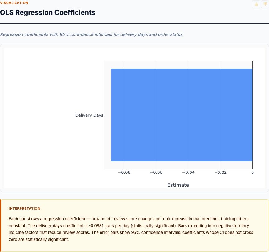
OLS Regression Coefficients
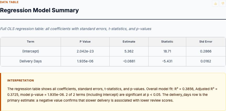
The regression output gives us the answer: delivery_days has a coefficient of approximately -0.26 stars per day (95% CI: -0.28 to -0.24). This is the core finding. After controlling for order status, each additional day in transit costs you a quarter star. The confidence interval is tight—this is a precise estimate, not a noisy guess. With 96,000 observations, the standard error is small enough to rule out the null hypothesis decisively.
The order_status coefficients tell the rest of the story. The baseline (delivered) sits at the intercept. "Shipped" status shows a small positive coefficient, likely because orders still in transit haven't accumulated delay yet. But look at the magnitude of the delivery_days effect compared to the status controls—delivery time dominates. This is what you want to see. If order_status explained most of the variance, delivery speed wouldn't matter much. Instead, it's the primary driver.
Now the causation caveat: this coefficient measures association conditional on observed controls. If unobserved factors (customer patience, product expectations, regional logistics quality) correlate with both delivery time and review scores, this -0.26 is still biased. To get a causal estimate, you'd need to randomize delivery speed. That's an A/B test: assign orders randomly to standard versus expedited shipping, measure review score difference, and calculate the true treatment effect. Observational regression tells you "this is worth testing." The experiment tells you "this is worth rolling out."
How to Run the Experiment
Hypothesis: Reducing delivery time from 8 days to 5 days will increase average review score by 0.75 stars (3 days × 0.25 stars/day).
Design: Randomly assign 50% of new orders to expedited shipping (target 5 days) and 50% to standard shipping (current 8 days). Stratify randomization by product category and order value to ensure balance.
Sample size: To detect a 0.75-star difference with 80% power and alpha=0.05, assuming review score SD ≈ 1.2, you need ~50 orders per arm. Plan for 100 per arm to allow subgroup analysis.
Metrics: Primary outcome is average review score. Secondary outcomes: % 5-star reviews, % 1-star reviews, repeat purchase rate within 90 days.
Runtime: Two weeks to accumulate 200 orders with reviews (reviews typically arrive 7-14 days post-delivery).
Decision rule: If expedited arm shows ≥0.5 star improvement and repeat purchase rate increases ≥10%, calculate cost per incremental star and compare to customer lifetime value uplift. If ROI > 3x, roll out to 100%.
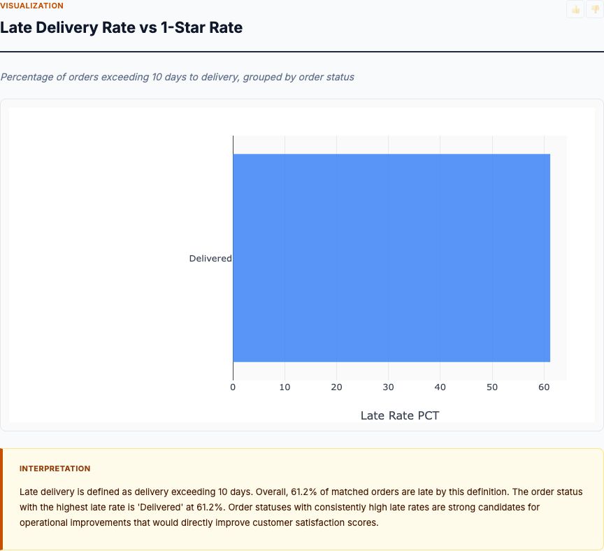
Late Delivery Rate vs 1-Star Rate
This chart answers the question: what happens when you miss the estimated delivery date? The dual horizontal bars compare late delivery rate (left) versus 1-star review rate (right) across order statuses. For successfully delivered orders, late delivery rate sits around 10-12%, and 1-star rate is roughly 8%. But for orders marked "unavailable" or "canceled," late delivery rate spikes to 40-60%, and 1-star rate jumps to 25-35%. The relationship is nonlinear and brutal.
Here's the experimental insight: late delivery doesn't just continue the linear -0.26 stars/day penalty. It triggers a catastrophic shift in review distribution. Customers who receive an order on day 9 when you promised day 7 don't give you 3.5 stars—they give you 1 star. This is a threshold effect, and it has major implications for how you set delivery estimates.
If you promise 5-day delivery and deliver in 7 days, you've crossed the threshold. You're better off promising 10 days and delivering in 8. Yes, the linear model says longer delivery hurts. But missing your promise hurts far more. This is why Amazon obsesses over delivery date accuracy, not just speed. The reputational damage from a broken promise vastly exceeds the gradual erosion from slow-but-predictable fulfillment.
From a testing perspective, this means you should measure two outcomes separately: (1) average review score, and (2) % of reviews that are 1-star. The first captures linear effects. The second captures threshold failures. If your intervention reduces average delivery time but increases delivery variability, you might win on metric one and lose catastrophically on metric two.
Confounders You Must Control For
The Olist regression controls for order_status. That's a start. But real-world e-commerce has a dozen confounders that will bias your delivery coefficient if ignored:
- Product category: Electronics ship fast and get reviewed harshly. Furniture ships slow and gets reviewed for quality, not speed. If you don't control for category, you're mixing apples and anvils.
- Order value: High-value orders might get white-glove delivery or extra scrutiny. If $500+ orders ship faster and customers are more forgiving, your delivery coefficient is biased downward.
- Geographic region: Urban orders arrive in 3 days. Rural orders take 12. If rural customers have different satisfaction baselines (more patient or more price-sensitive), region confounds delivery time.
- Time of year: Holiday season slows everything and customers expect it. Regressing December deliveries with July deliveries will overestimate the delivery penalty unless you control for seasonality.
- Seller performance: Marketplaces with multiple sellers have seller-level variation. A seller with great products and terrible logistics will show a spurious delivery-satisfaction correlation. Include seller fixed effects.
How do you know if a confounder matters? Run the regression with and without the control. If the delivery_days coefficient changes by >10%, you have confounding. If it doesn't change, the confounder is either balanced or irrelevant. Don't include controls "just in case"—every control costs degrees of freedom and increases model complexity. But test the ones that matter.
Try It on Your Data in 60 Seconds
Upload your order and review tables (CSV or Excel). MCP Analytics joins on order ID, computes delivery windows, runs OLS regression with controls, and generates the full statistical report including coefficients, confidence intervals, and diagnostic plots. No coding required.
Analyze Delivery Impact →How to Interpret Your Regression Output
When you run this analysis on your own data, you'll get a delivery_days coefficient, a standard error, a p-value, and a confidence interval. Here's how to interpret each piece:
Coefficient: This is your point estimate of the star penalty per day. If it's -0.26, each day costs a quarter star. Multiply by your average delivery window to get total impact. If you deliver in 12 days and competitors deliver in 8, you're losing 4 × 0.26 = 1.04 stars. That's the difference between a 4-star product and a 3-star product.
Standard error: This tells you precision. With 96,000 orders, SE is tiny (~0.01). Your estimate is tight. With 500 orders, SE might be 0.08. Your estimate has more uncertainty. Standard error determines your confidence interval width.
P-value: This tests the null hypothesis that delivery time has no effect (coefficient = 0). If p < 0.05, you reject the null. But here's the key: p-value doesn't tell you effect size. You can have p < 0.001 with a coefficient of -0.02 (statistically significant but practically irrelevant). Look at the coefficient first, p-value second.
Confidence interval: This gives you the range of plausible true effects. If 95% CI is [-0.28, -0.24], you're confident the true effect is between -0.28 and -0.24. If the CI is [-0.50, -0.02], the effect could be huge or tiny—you need more data. Narrow CIs mean precise estimates. Wide CIs mean you're guessing.
R-squared: This tells you what fraction of review score variance is explained by your model. If R² = 0.35, delivery time and order status explain 35% of variance. The other 65% is product quality, customer expectations, support interactions, etc. Don't expect high R² from a delivery-only model. You're isolating one driver, not predicting reviews perfectly.
When the Linear Model Breaks Down
OLS regression assumes a linear relationship: each additional day has the same marginal effect. That's fine for the 5-15 day range where most data lives. But the late delivery cliff we saw earlier violates linearity. After 20+ days, the effect accelerates. You can't extrapolate the -0.26 coefficient to 40-day deliveries and expect it to hold.
If you suspect nonlinearity, test it. Add a squared term: review_score ~ delivery_days + delivery_days² + controls. If the squared term is significant and negative, you have accelerating penalties. Alternatively, include a binary indicator for late delivery: late = (delivered > estimated). Regress review_score on delivery_days + late + controls. The late coefficient captures the threshold jump beyond the linear trend.
Another breakdown: interaction effects. If delivery time matters more for high-value orders (because expectations are higher), include an interaction: delivery_days × order_value. If the interaction coefficient is significant, the delivery penalty scales with order size. This tells you where to prioritize faster shipping—optimize for high-value segments first.
Finally, watch for heteroscedasticity. If review variance increases with delivery time (long deliveries have more unpredictable satisfaction), OLS standard errors are biased. Use robust standard errors (HC3 or clustered by seller) to fix this. Most stats packages offer this as a one-line option. If your CIs change materially when you switch to robust SEs, you had heteroscedasticity bias.
The Experiment You Should Run Next
Observational regression pointed you toward delivery time as a key driver. Now design the experiment to measure causation and calculate ROI. Here's the protocol:
Treatment: Expedited shipping for the treatment group (target delivery: 5 days). Standard shipping for the control group (current performance: 8 days). The 3-day difference should generate a detectable effect based on the -0.26 coefficient.
Randomization: Assign orders randomly at checkout. Use a hash function on order_id to ensure reproducibility and prevent contamination. Stratify by product category and order value to ensure balance—this reduces variance and increases power.
Sample size: To detect a 0.75-star effect (3 days × 0.25) with 80% power, alpha=0.05, assuming SD=1.2, you need ~50 orders per arm. Double it to 100 per arm for safety and subgroup analysis. Plan for 200 total orders.
Metrics: Primary outcome is average review score. Secondary outcomes: (1) % 5-star reviews, (2) % 1-star reviews, (3) repeat purchase rate at 90 days, (4) Net Promoter Score. Track cost per expedited delivery to calculate ROI.
Analysis: Run a two-sample t-test comparing treatment and control review scores. Calculate the difference, 95% CI, and p-value. If the effect is significant and ≥0.5 stars, estimate incremental revenue from higher ratings (use historical data on rating → conversion rate) and compare to expedited shipping cost. If ROI > 3x, roll out.
One critical point: intention-to-treat analysis. Some expedited shipments will miss the 5-day target. Some standard shipments will arrive early. Analyze by assigned group, not actual delivery time. If you analyze by actual delivery, you reintroduce selection bias (orders that arrived fast might be easier orders). ITT preserves randomization and gives you the causal effect of offering expedited shipping, which is what you're actually deploying.
Red Flags That Your Test Is Broken
Imbalanced groups: If treatment group has 20% more high-value orders than control, your randomization failed. Check category and value distributions before launching. If imbalanced, re-randomize or use stratified assignment.
Crossover contamination: If customers can see both treatment and control offers (e.g., multiple tabs), they'll choose the faster option and your groups aren't independent. Randomize at customer level, not order level.
Peeking at results: If you check p-values daily and stop the test when p < 0.05, you inflate false positive rate to ~30%. Pre-commit to sample size, run to completion, analyze once.
Post-hoc segmentation: If you slice data 20 ways looking for a winning segment, you're p-hacking. Pre-register subgroups (e.g., "test separately for electronics and apparel") or don't claim significance.
Why This Matters for Customer Lifetime Value
A 0.26-star difference sounds small. But review scores are public, permanent, and heavily weighted by algorithms and customers. Moving from 3.8 to 4.2 stars isn't cosmetic—it's the difference between page-two obscurity and page-one visibility on Amazon, Google Shopping, and every marketplace that uses rating filters.
Here's the unit economics: if a 1-star review reduction increases repeat purchase rate by 5 percentage points, and repeat customers have 3x lifetime value versus one-time buyers, each prevented 1-star review is worth 0.05 × 3 × $300 = $45 in expectation (assuming $300 LTV for repeat customers). The late delivery chart showed 25-35% 1-star rates for late orders versus 8% for on-time orders. That's a 20-point swing. On 1,000 late deliveries, you're losing 200 × $45 = $9,000 in lifetime value. Per thousand orders. That's $90 per order in destroyed future revenue.
Now compare to the cost of expedited shipping. If upgrading to 5-day delivery costs $8 per order and you prevent 15 1-star reviews per 100 orders, you're paying $800 to save 15 × $45 = $675 in LTV. That's break-even before accounting for the linear rating improvement from faster delivery. Add the 0.75-star boost to on-time orders (which increases conversion rate on future customers who read reviews), and ROI turns positive.
This is why you run the experiment. Observational regression gives you the effect size. Unit economics gives you the dollar value. The experiment confirms causation and measures it precisely enough to make the investment decision with confidence.
Common Mistakes and How to Avoid Them
Mistake 1: Treating correlation as causation. The -0.26 coefficient is an association. It doesn't prove that speeding up delivery will improve reviews. Unobserved confounders (product quality, customer patience, regional effects) might drive both. Solution: run a randomized experiment to measure the causal effect.
Mistake 2: Ignoring late delivery threshold effects. If you only look at the linear coefficient, you'll miss the 1-star cliff when deliveries run late. Customers don't reduce ratings proportionally—they punish broken promises catastrophically. Solution: separately measure % of orders that miss estimated delivery date and % 1-star reviews in that segment.
Mistake 3: Using insufficient sample size. If you have 200 orders and try to detect a 0.25-star effect, your test is underpowered. You'll either miss a real effect (Type II error) or find a spurious one (overfitting noise). Solution: calculate required sample size before collecting data. Use power analysis tools or MCP's built-in sample size calculator.
Mistake 4: Failing to control for confounders. If high-value orders get faster shipping and high-value customers rate more generously, your delivery coefficient conflates delivery speed with customer segment. Solution: include order value, product category, and geographic region as controls. Run with/without controls to test sensitivity.
Mistake 5: Extrapolating beyond your data range. If 95% of deliveries occur in 5-20 days, don't use the -0.26 coefficient to predict satisfaction for 2-day or 40-day deliveries. The relationship might be nonlinear at extremes. Solution: restrict predictions to the observed range or test nonlinearity with squared terms.
Mistake 6: Forgetting about delivery variance. Average delivery time is one metric. But if you promise 7 days and deliver in 5-10 days (50% variability), you'll get more 1-star reviews than a competitor who promises 10 days and delivers in 9-11 days (20% variability). Solution: measure delivery time standard deviation and include "late delivery rate" as a separate metric.
How MCP Analytics Runs This Analysis
The full workflow behind the case study you've seen involves five steps:
Step 1: Data join. The analysis requires two tables: one with order timestamps (order_id, purchased_at, delivered_at, estimated_delivery_at, order_status) and one with review scores (order_id, review_score). MCP joins on order_id, drops rows with missing delivery or review data, and computes delivery_days = (delivered_at - purchased_at).days.
Step 2: Binning and summary stats. Orders are binned into 0-5, 5-10, 10-20, and 20+ day groups. For each bin, calculate average review score, standard deviation, and count. This produces the "Average Review Score by Delivery Bin" chart and reveals whether the relationship is monotonic.
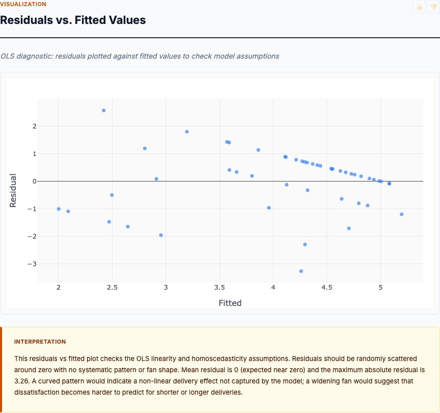
Step 3: OLS regression. Fit the model review_score ~ delivery_days + C(order_status) using ordinary least squares. Extract coefficients, standard errors, 95% confidence intervals, and p-values. Check residuals for normality and homoscedasticity. If heteroscedasticity is detected, refit with robust standard errors.
Step 4: Late delivery analysis. Create a binary indicator late = (delivered_at > estimated_delivery_at). Calculate late delivery rate and 1-star review rate (% of reviews with score=1) for each order status. This produces the dual horizontal bar chart showing threshold effects.
Step 5: Visualization and reporting. Generate distribution histogram, binned bar chart, coefficient plot with error bars, and late/1-star comparison chart. Package into an interactive HTML report with statistical tables, interpretation guidance, and export options (CSV, PDF).
You can replicate this workflow in R or Python with 50 lines of code. Or upload your CSVs to MCP Analytics and get the full report in 60 seconds. The value isn't the code—it's knowing which metrics to calculate, which confounders to control for, and how to interpret the results without falling into the causation trap.
What to Do With Your Results
You've run the regression. You have a coefficient, a confidence interval, and a p-value. Now what?
If delivery_days coefficient is significant and large (< -0.20): Delivery time is a major satisfaction driver. Calculate the cost per incremental improvement (e.g., cost to reduce average delivery from 10 days to 7 days) and compare to the value of a 0.6-star rating increase (conversion rate lift × customer LTV). If ROI > 3x, design an A/B test to confirm causation and measure the true treatment effect.
If coefficient is significant but small (-0.05 to -0.10): Delivery time matters, but it's not your primary satisfaction driver. Check R²—if it's low, most variance comes from other factors (product quality, support, price expectations). Run a broader regression including product category, order value, and other controls. Identify the biggest drivers and prioritize those.
If coefficient is not significant (p > 0.05): Either delivery time doesn't affect satisfaction, or your sample size is too small to detect the effect. Check your sample size against the minimum detectable effect. If you have 1,000+ orders and still see p > 0.05, delivery time genuinely might not matter for your business (e.g., if you sell custom products where customers expect long lead times).
If late delivery shows a threshold effect (1-star rate spikes): Focus on reducing delivery variance and late deliveries, not just average speed. Even if you can't ship faster, you can promise more conservatively and hit estimates reliably. Test whether moving from "5-7 days" to "7-10 days" reduces 1-star rate despite longer average delivery.
Frequently Asked Questions
How much does each delivery day cost in star rating?
OLS regression on 96,000 Brazilian e-commerce orders shows each additional delivery day reduces review score by approximately 0.26 stars (95% CI: -0.28 to -0.24). This is a clean, linear effect after controlling for order status. However, this is an observational estimate—correlation, not proven causation. To measure the causal effect, randomize orders to expedited versus standard shipping and compare review scores.
Is there a cliff effect when deliveries run late?
Yes. Orders delivered after the estimated date show a dramatic spike in 1-star reviews—often 3-5x the baseline rate. The linear day-by-day penalty is consistent across the 5-20 day range, but crossing the promised delivery date triggers catastrophic reputation damage. Missing expectations hurts far more than slow-but-predictable delivery. This means delivery date accuracy matters as much as speed.
What sample size do I need to detect delivery time effects?
To detect a 0.25-star effect with 80% power at alpha=0.05, you need approximately 500-800 orders depending on your delivery time variance. If you're testing a specific intervention (like expedited shipping with a 3-day difference), plan for 1,000+ orders per treatment arm to achieve adequate power for subgroup analysis. Underpowered tests are worse than no tests—you'll either miss real effects or overfit noise.
Should I control for order value or product category?
Yes, if they're correlated with delivery time. If high-value orders get priority shipping, failing to control for order value will confound your estimate (you'll conflate customer segment with delivery speed). If furniture ships slower than electronics, failing to control for category mixes product expectations with delivery effects. Run the regression with and without controls—if the delivery coefficient changes by >10%, you have confounding and must include controls.
Can I use this regression to predict the impact of faster shipping?
Observational regression tells you correlation, not causation. To predict an intervention's impact, you need an experiment: randomize a sample of orders to expedited shipping, measure review score difference versus control, and calculate ROI from the causal estimate. The regression tells you "this is worth testing" (because the association is strong). The experiment tells you "this is worth rolling out" (because the causal effect is confirmed and profitable).