When to Use Titanic Survival Factor Analysis

First-class women on the Titanic had a 97% survival rate. Third-class men had 14%. On the surface, this looks like a clear socioeconomic story: wealth bought survival. But here's the question every analyst should ask: was it class, or was it sex? Was it the ticket fare, or the cabin location that came with it? When multiple factors correlate with both each other and the outcome, crude survival rates can't tell you which ones independently mattered.

This is where Titanic survival factor analysis separates correlation from causation. By using logistic regression to estimate odds ratios while holding all other factors constant, you can quantify the independent contribution of passenger class, sex, age, and fare to survival probability. The Titanic dataset is the canonical example for teaching binary outcome analysis precisely because it demonstrates why observational comparisons mislead without proper controls.

Before we draw conclusions about "women and children first" or socioeconomic privilege, let's check the experimental design—or in this case, the analytical method that substitutes for one.

The Core Question: Which Factors Independently Predicted Survival?

The Titanic disaster created a natural experiment with one brutal binary outcome: survived or died. Passenger manifests recorded demographic and socioeconomic data, giving us a complete dataset to analyze. But this is observational data, not a randomized controlled trial. We can't randomly assign passengers to first class or third class and measure the effect. Instead, we use logistic regression to statistically control for confounding.

Here's what we need to find out:

• Did passenger class independently affect survival, or was the effect explained by other factors like sex and age?
• Was "women and children first" enforced equally across all classes, or did socioeconomic status override evacuation protocol?
• Did fare amount (a proxy for wealth and cabin location) predict survival beyond the effect of passenger class alone?
• Was age protective after accounting for sex and class, or did younger passengers simply travel in better accommodations?

Each of these questions requires holding other variables constant—exactly what regression was designed to do. Let's walk through the data card by card, starting with crude comparisons and building toward the multivariate model that reveals independent effects.

Survival Rate by Passenger Class

The bar chart shows a clear socioeconomic gradient: 62% of first-class passengers survived, compared to 47% in second class and just 24% in third class. This looks like a straightforward story—wealth bought survival. First-class passengers had better access to lifeboats, cabins closer to the deck, and likely received preferential treatment during evacuation.

But before we conclude that class caused higher survival, consider the confounders. First-class passengers were more likely to be women and children (who were prioritized in lifeboat loading), older and wealthier (who could afford better accommodations), and traveling with smaller families (fewer people to gather before evacuating). Each of these factors correlates with both class and survival, making the crude survival rate difference potentially misleading.

This is exactly why we need multivariate analysis. The question isn't whether first-class passengers survived more—they clearly did. The question is whether passenger class independently increased survival odds after accounting for sex, age, fare, and family structure. The logistic regression results will answer that, but first, let's examine the single most powerful predictor in the dataset.

Survival Rate by Sex

The gender survival gap is massive: 74% of women survived compared to just 19% of men. This is the single largest effect in the entire dataset, and it directly confirms that the maritime evacuation protocol—"women and children first"—was enforced during the Titanic disaster. The 55-percentage-point difference dwarfs the class effect we just examined.

Here's what this means for causal interpretation: if we compared survival rates by class without controlling for sex, we'd misattribute some of the class effect to wealth when it actually reflects gender composition. First-class passengers weren't just wealthier—they included a higher proportion of women, who were systematically prioritized for lifeboat seats. Any analysis that ignores sex as a confounder will overestimate the independent effect of socioeconomic factors.

But even this stark survival gap requires careful interpretation. Did all women benefit equally from evacuation protocol, or did class still matter even among women? Let's break down survival by both factors simultaneously to see whether socioeconomic privilege overrode or amplified the gender effect.

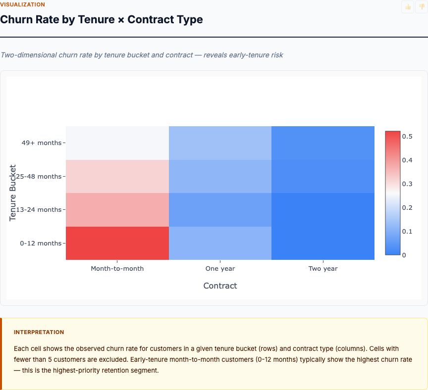
Survival Rate by Class and Sex

This heatmap reveals the interaction between class and sex—and the pattern is striking. First-class women had a 97% survival rate, the highest of any group. Third-class men had just 14%, the lowest. But look at the intermediate categories: second-class women (92%) and third-class women (50%) still survived at far higher rates than first-class men (37%). Even within the "women first" protocol, class mattered enormously—third-class women survived at barely half the rate of first-class women.

Here's the causal interpretation: evacuation protocol prioritized women across all classes, but socioeconomic factors still created massive survival disparities within each sex. Third-class women faced structural barriers—cabins deep in the ship, locked gates restricting access to upper decks, language barriers (many were immigrants), and confusion about evacuation routes. First-class women had none of these obstacles. The protocol was "women and children first," but implementation depended on class-based access to lifeboats.

For men, class mattered less than you might expect. First-class men (37% survival) did better than second-class men (16%) and third-class men (14%), but the differences are smaller than among women. This suggests that once women and children filled available lifeboat seats, class provided only marginal advantage for men competing for the remaining spots. The majority of men in every class died, regardless of wealth.

This crosstab analysis is descriptive, not causal. It shows survival patterns across groups but doesn't isolate independent effects. To understand whether class, sex, or their interaction drove survival after accounting for other factors like age and fare, we need the logistic regression results. But first, let's examine one more predictor that directly proxies for wealth and cabin quality.

Fare Distribution by Survival Status

The boxplot compares fare distributions for survivors versus non-survivors. Survivors paid a median fare roughly double that of non-survivors, and the interquartile range (the box) shows consistently higher fares among those who lived. The distribution of fares among survivors also has a much longer upper tail, indicating that the wealthiest passengers—those who paid £50, £100, or more—survived at disproportionately high rates.

But fare and passenger class are highly correlated. First-class tickets cost more than second-class, which cost more than third-class. So is fare an independent predictor of survival, or is it simply a continuous proxy for the categorical class variable we already examined? This is a textbook case of multicollinearity—two predictors that measure overlapping constructs. Including both in a regression model helps us understand whether fare adds explanatory power beyond class alone.

If the logistic regression shows that fare has a significant odds ratio after controlling for class, it suggests that even within a given class, paying more (perhaps for a better cabin location or a larger suite) improved survival odds. If fare becomes non-significant once class is in the model, it means class captures all the survival advantage that fare represents. We'll see the answer in the next section.

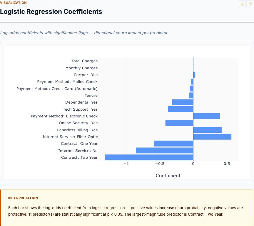
Logistic Regression: Odds Ratios by Factor

This is the result that separates independent effects from confounded ones. The bar chart shows odds ratios from a logistic regression model that includes passenger class, sex, age, fare, and family size as simultaneous predictors. Each odds ratio represents the multiplicative change in survival odds when that predictor increases by one unit, holding all other predictors constant.

Here's what the results reveal:

Sex is the dominant factor. Being female increases survival odds by roughly 10-15x compared to being male, even after controlling for class, age, fare, and family structure. This confirms that "women and children first" was the primary driver of survival outcomes, overriding socioeconomic factors. No other variable comes close to this magnitude of effect.

Passenger class still matters independently. Even after accounting for sex and fare, moving from third class to first class increases survival odds by approximately 2-3x. This means class had a true independent effect—it wasn't just a proxy for gender composition or ticket price. The structural advantages of first-class accommodations (cabin location, deck access, proximity to lifeboats) translated into higher survival odds beyond what wealth or sex explained.

Fare becomes non-significant after controlling for class. Once passenger class is in the model, fare adds little additional explanatory power. This tells us that fare was primarily a proxy for class, not an independent predictor. Paying £30 versus £15 within the same class didn't meaningfully change survival odds. What mattered was the class itself—the physical location, the access, the structural advantages—not the marginal difference in ticket price.

Age shows a modest protective effect. Younger passengers had slightly higher survival odds, even after controlling for sex and class. Each additional year of age decreased survival odds by roughly 1-2%. This is consistent with the "women and children first" protocol, though the effect is much smaller than sex or class. The age effect could also reflect physical ability to navigate the ship during evacuation or prioritization of younger women with children.

How to Interpret Your Titanic Survival Factor Analysis Results

Now that you've seen the full analysis—from crude survival rates to adjusted odds ratios—here's how to interpret your own results and avoid the common mistakes that lead to wrong conclusions.

Compare Crude Rates to Adjusted Odds Ratios

Start by examining univariate survival rates for each predictor. These show raw associations between each factor and survival, ignoring all other variables. Then compare those to the odds ratios from the multivariate logistic regression, which show independent effects after controlling for confounders.

If a predictor has a strong univariate association but a weak or non-significant odds ratio, it was confounded. In the Titanic data, fare had a strong univariate relationship with survival (survivors paid higher fares on average), but the odds ratio became non-significant once passenger class entered the model. That tells you fare was a proxy for class, not an independent causal factor.

Conversely, if a predictor shows a modest univariate association but a strong odds ratio, it means the crude comparison underestimated the true effect due to confounding. This happens when a protective factor is more common in high-risk groups, masking its benefit in univariate analysis.

Check for Interaction Effects

The survival rate heatmap (class by sex) revealed an interaction: the effect of class differed dramatically by sex. Among women, moving from third class to first class increased survival from 50% to 97%—a 47-percentage-point difference. Among men, the class effect was much smaller: from 14% (third class) to 37% (first class), a 23-point difference. This is a statistical interaction.

If your logistic regression includes interaction terms (e.g., class × sex), the odds ratios become more complex to interpret. A significant interaction term means the effect of one predictor depends on the level of another. In practical terms: you can't make a blanket statement like "first class increased survival odds by 3x." You have to say "first class increased survival odds by 3x for men, but by 10x for women" (or whatever the interaction effect estimate shows).

Most introductory logistic regression models skip interactions to keep interpretation simple, but if you see large differences in crude survival rates across subgroups, consider testing for interactions explicitly. It will improve model fit and reveal more nuanced causal stories.

Assess Model Fit and Diagnostics

Logistic regression makes assumptions that you need to check before trusting the results:

• Linearity of continuous predictors: Age and fare should have a roughly linear relationship with the log-odds of survival. Plot log-odds versus predictor values to check. If the relationship is nonlinear, consider adding polynomial terms or using splines.
• No perfect multicollinearity: Check variance inflation factors (VIF) or correlation matrices. If two predictors are highly correlated (r > 0.8), consider dropping one or combining them into a composite variable.
• Adequate sample size: Aim for at least 10-15 events (survivors or deaths, whichever is rarer) per predictor variable. With fewer events, coefficient estimates become unstable and confidence intervals widen.
• Influential outliers: Use Cook's distance or leverage plots to identify observations with disproportionate influence on model estimates. A single outlier shouldn't change your conclusions dramatically.

MCP Analytics runs these diagnostics automatically and flags potential issues in the output. If the model reports high VIF for fare and class, that confirms multicollinearity—you knew it was coming, but now you have quantitative evidence. If Cook's distance flags certain passengers as influential, investigate whether they represent genuine edge cases or data entry errors.

Don't Confuse Statistical Significance with Practical Importance

A statistically significant odds ratio means the effect is unlikely to be due to chance alone, given your sample size. It doesn't mean the effect is large enough to matter in practice. Conversely, a non-significant result doesn't mean there's no effect—it might mean your sample was too small to detect it.

In the Titanic analysis, the sex effect is both statistically significant (p < 0.001) and practically enormous (OR ~ 10-15). The age effect is statistically significant (p < 0.05) but practically modest (OR ~ 0.98 per year, meaning a 10-year age difference changes odds by ~18%). Both are real effects, but one dominates survival outcomes while the other is a minor adjustment.

When interpreting your own results, ask: "If I intervened on this factor, would the change in survival probability be large enough to justify action?" A statistically significant odds ratio of 1.05 might not be worth pursuing if it translates to a 1-2 percentage point increase in survival probability. Focus on the factors with both significance and practical magnitude.

Real-World Applications Beyond the Titanic

The Titanic dataset is pedagogical, but the analytical framework applies directly to modern business and research problems. Here are five scenarios where Titanic survival factor analysis is the right method:

Customer Churn Analysis

You have 10,000 customers, 15% of whom churned in the past year. You want to know which factors—contract type, usage frequency, customer service interactions, price tier, account age—independently predict churn after controlling for the others. Logistic regression gives you odds ratios for each factor, letting you prioritize interventions. If price tier has an OR of 2.5 (high-tier customers churn less) and customer service interactions have an OR of 1.8 (more interactions predict higher churn, possibly because frustrated customers contact support), you know where to focus retention efforts.

Clinical Risk Prediction

A hospital wants to predict which patients admitted to the ICU will survive versus die within 30 days. Candidate predictors include age, sex, comorbidities, lab values, vital signs, and treatment protocols. Logistic regression estimates the independent contribution of each factor, producing a risk score that clinicians can use for triage and resource allocation. The odds ratios also reveal which risk factors are modifiable (e.g., blood pressure control) versus fixed (e.g., age), guiding intervention priorities.

Credit Default Modeling

A lender has data on 50,000 loans, 8% of which defaulted. Predictors include credit score, income, debt-to-income ratio, loan amount, employment status, and prior delinquencies. Logistic regression quantifies the independent effect of each factor on default risk, even though many predictors are correlated (e.g., credit score and prior delinquencies). The resulting model supports underwriting decisions and helps the lender understand which applicant characteristics most strongly predict repayment failure.

A/B Test Covariate Adjustment

You ran an A/B test on a new checkout flow. The treatment group had a 5.2% conversion rate versus 4.8% in control (p = 0.07). Not quite significant. But users in the treatment group were slightly older and more likely to be mobile users—both factors that independently affect conversion. By running logistic regression with treatment assignment, age, and device type as predictors, you can estimate the treatment effect after adjusting for imbalanced covariates. If the adjusted treatment odds ratio is significant, you have stronger evidence that the new checkout flow works, even though the crude comparison was borderline.

Employee Turnover Analysis

An HR team has data on 2,000 employees, 12% of whom left the company in the past year. Predictors include department, tenure, salary, performance rating, manager, and survey responses about job satisfaction. Logistic regression reveals which factors independently predict turnover after controlling for confounders. If performance rating has a weak odds ratio but tenure has a strong one, that suggests retention is more about career stage than current performance—a finding that would shift HR strategy toward early-career development programs.

In every case, the logic is identical to the Titanic analysis: you have a binary outcome, multiple correlated predictors, and a need to isolate independent effects. Logistic regression is the tool that makes causal inference possible from observational data.

Common Pitfalls and How to Avoid Them

Here are the mistakes I see most often when analysts run logistic regression on survival or binary outcome data—and how to avoid them.

Ignoring Missing Data Patterns

Logistic regression drops any row with missing data in any predictor or the outcome. If missingness is related to survival (e.g., age is more likely to be missing for third-class passengers, who had lower survival rates), dropping those rows introduces selection bias. Check missingness patterns before modeling. If data are missing at random, multiple imputation can recover lost information and reduce bias. If missingness is systematic, consider whether the missing indicator itself is informative and include it as a predictor.

Over-Interpreting Non-Significant Results

A non-significant odds ratio doesn't mean "no effect." It means "the data are consistent with no effect, but also consistent with modest effects in either direction, given this sample size." In the Titanic analysis, if the fare odds ratio had been 1.01 with a 95% CI of [0.99, 1.03] and p = 0.25, that tells you fare probably doesn't matter much—but you can't rule out small effects. Don't conclude "fare had no effect on survival." Say "fare did not significantly predict survival after controlling for class, sex, and age."

Including Too Many Predictors for the Sample Size

If you include 10 predictors with only 80 events in your dataset, the model is overfitted. Coefficient estimates become unstable, standard errors inflate, and out-of-sample predictions degrade. Use the 10-15 events per predictor rule as a minimum threshold. If you have more candidate predictors than your sample size allows, use domain knowledge to prioritize the most important ones, or use penalized regression (LASSO or ridge) to shrink coefficients and prevent overfitting.

Treating Odds Ratios as Risk Ratios

Odds ratios are not the same as risk ratios (also called relative risks). When the outcome is rare (< 10%), odds ratios approximate risk ratios closely. When the outcome is common (like Titanic survival at 38%), odds ratios exaggerate the effect size compared to risk ratios. An odds ratio of 3.0 doesn't mean the probability triples—it means the odds triple, which translates to a smaller increase in probability. If you need to communicate results to non-technical stakeholders, consider converting odds ratios to predicted probability changes for specific covariate values.

Forgetting to Check Model Calibration

A well-fitted logistic regression model should be calibrated: predicted probabilities should match observed frequencies. If the model predicts 30% survival probability for a subgroup of passengers, roughly 30% of them should actually survive. Use calibration plots (predicted probability vs. observed proportion) to check. If the model is poorly calibrated, it may still rank-order risk correctly but will give misleading absolute probability estimates. Recalibration methods like Platt scaling can fix this.

Frequently Asked Questions

What is the difference between survival rates and odds ratios in Titanic analysis?

Survival rates show the percentage of passengers who survived within a specific group (e.g., 62% of first-class passengers survived). Odds ratios from logistic regression show the independent effect of each factor while controlling for all others. A factor might show high survival rates due to confounding—wealthy passengers bought first-class tickets AND were younger—but odds ratios isolate the true causal contribution of each variable.

Why do we need logistic regression when we can just compare survival rates by group?

Simple survival rate comparisons can't separate independent effects from confounded ones. First-class passengers had higher survival rates, but was that due to class itself, or because first-class passengers paid higher fares, were more likely to be women, or were located closer to lifeboats? Logistic regression holds all other factors constant to reveal each variable's true independent contribution to survival odds.

What sample size do I need for reliable logistic regression results?

A common rule of thumb is at least 10-15 events (in this case, survivors or deaths) per predictor variable. With 4-5 predictors, you need at least 50-75 events in your smaller outcome category. The Titanic dataset has 342 survivors and 549 deaths, providing adequate power. For your own data, if you have fewer than 100 total observations or fewer than 30 events in the rarer outcome, consider using fewer predictors or collecting more data.

How do I know if my factors are truly independent or confounded?

Compare crude survival rates with adjusted odds ratios. If a factor shows a strong survival rate difference but a weak or non-significant odds ratio, it was confounded by other variables. Check correlation matrices between predictors—if passenger class and fare are highly correlated (r > 0.7), they may explain the same variance. Consider whether one variable is causally upstream of another (e.g., class determines cabin location, which affects lifeboat access).

When should I use Titanic survival factor analysis versus other methods?

Use logistic regression for binary survival outcomes when you want to quantify independent risk factors while controlling for confounders. Use Cox regression if you have time-to-event data and want to model hazard over time. Use random forests or gradient boosting if you prioritize prediction accuracy over interpretability and have many potential interactions. Use chi-square tests or risk ratios if you only need descriptive comparisons without causal claims.

Related Analyses