When to Use Advertising Spend Effectiveness by Channel

Your CMO just asked which advertising channel drives the most sales. TV spend and sales both increased this quarter—correlation 0.78. Looks like TV is the winner, right? Not so fast. Radio spend also increased. Newspaper spend increased. Even your organic social activity ramped up. Which channel actually caused the lift?

This is the attribution problem every marketer faces. Simple correlations mislead because multiple channels move together. What you need is multiple linear regression—a statistical method that isolates each channel's independent contribution by controlling for all other channels simultaneously. It answers the critical question: If I increase TV spend by $1,000 while holding Radio and Newspaper constant, how much do sales increase?

Before we draw conclusions from correlation, let's check the experimental design. Or in this case, the observational design—because most marketing data comes from campaigns you already ran, not controlled experiments. That means we need regression to tease apart confounded effects.

The Attribution Problem: Why Single-Channel Analysis Fails

Imagine you're analyzing 200 weeks of advertising data. Each week you spent money on TV, Radio, and Newspaper ads. Sales varied from $1,600 to $27,000 per week. Your first instinct: calculate correlation between each channel and sales.

Here's what you find:

• TV spend correlates with sales at r = 0.78 (strong positive)
• Radio spend correlates with sales at r = 0.58 (moderate positive)
• Newspaper spend correlates with sales at r = 0.23 (weak positive)

The naive conclusion: TV is the winner, invest everything there. But correlation measures association, not causation. TV spend might correlate with sales because you tend to increase all channels simultaneously during high-demand seasons. Or because TV spend tracks with Radio spend (if you run integrated campaigns). Or because both TV and sales are driven by a third variable—say, product quality improvements over time.

The fundamental issue: when multiple predictors correlate with both the outcome and each other, simple correlation conflates direct effects with confounding. You can't isolate TV's true contribution without controlling for Radio and Newspaper.

How Multiple Regression Isolates Channel Effects

Multiple linear regression fits this equation to your data:

Sales = β₀ + β₁(TV) + β₂(Radio) + β₃(Newspaper) + ε

Where:

• β₀ (intercept): Expected sales when all channels spend $0
• β₁ (TV coefficient): Sales change per $1,000 increase in TV, holding Radio and Newspaper constant
• β₂ (Radio coefficient): Sales change per $1,000 increase in Radio, holding TV and Newspaper constant
• β₃ (Newspaper coefficient): Sales change per $1,000 increase in Newspaper, holding TV and Radio constant
• ε (residual): Unexplained variation

The "holding constant" clause is the key. Regression finds the unique contribution of each channel after accounting for the others. It's partial correlation—the correlation between TV and sales after removing the influence of Radio and Newspaper.

Here's the practical translation: β₁ tells you the sales lift from a $1,000 increase in TV spend in a week where Radio and Newspaper budgets don't change. That's the isolated TV effect.

When to Use This Analysis: The Decision Checklist

Use advertising spend effectiveness regression when:

1. You have historical spend data across multiple channels (minimum 100-200 observations for stable estimates with 3 predictors)
2. You want to isolate each channel's independent contribution rather than just overall correlation
3. Your channels vary independently enough to separate their effects (check multicollinearity—correlation between predictors should be below 0.7-0.8)
4. You're making budget allocation decisions and need to know ROI per channel
5. You haven't run randomized experiments and need to learn from observational campaign data

Don't use this analysis when:

• You have fewer than 50-100 observations (coefficients will be unstable)
• Your channels are perfectly collinear—you always spend the same proportion on TV and Radio (regression can't separate their effects)
• You expect significant interaction effects (TV amplifies Radio's effectiveness)—standard regression assumes additive effects
• You have time-series data with strong autocorrelation or seasonality (use time-series regression or ARIMA instead)

Reading the Report: Card by Card

Let's walk through an actual analysis of 200 weeks of advertising data. Each section below shows a card from the regression report, with the insight it reveals and how to interpret the numbers.

Spend Distribution by Channel

Before running regression, inspect the distribution of your predictors. This box plot shows TV spend ranges from near $0 to $300K, with a median around $150K. Radio spans $0 to $50K, median ~$25K. Newspaper runs $0 to $115K, median ~$30K.

What to look for: Outliers and skewness. If you see extreme outliers (e.g., one week with 10x normal spend), they can distort regression coefficients. Consider whether those weeks represent true variation you want to model or data errors you should exclude. Heavy skewness may warrant log-transforming spend variables, though linear models often handle moderate skewness well.

In this dataset, distributions are reasonably symmetric with some high-spend outliers. That's fine—those outlier weeks provide valuable information about high-budget effectiveness. If you had 95% of weeks at $100K TV spend and one week at $500K, that single observation would have disproportionate leverage. Here the variation is spread out enough to trust the estimates.

Practical check: Confirm you have sufficient variation in each channel. If TV spend was constant at $150K every week, the regression can't estimate its effect—you need variation to measure impact. This dataset passes: each channel varies substantially across weeks.

Spend & Sales Correlation Matrix

This heatmap reveals two critical patterns: how each channel correlates with sales (top row) and how channels correlate with each other (off-diagonal cells).

Correlation with sales: TV shows the strongest correlation with sales (0.78), followed by Radio (0.58) and Newspaper (0.23). As discussed earlier, these are crude associations—they don't isolate each channel's independent effect. But they set a baseline: if regression coefficients diverge dramatically from these correlations, investigate why.

Multicollinearity check: TV-Radio correlation is 0.05 (near zero), TV-Newspaper is 0.06, Radio-Newspaper is 0.35. All well below the 0.7-0.8 threshold where multicollinearity becomes problematic. This is excellent news—it means the channels vary independently enough that regression can cleanly separate their effects.

Contrast with a problematic scenario: imagine TV-Radio correlation was 0.92 because you always spend $2 on Radio for every $10 on TV. Then regression struggles to distinguish their effects—it can estimate the combined TV+Radio impact, but not each individually. The coefficients would have huge standard errors and flip signs based on small data changes. Low multicollinearity here means stable, trustworthy estimates.

What if you see high multicollinearity? Three options: (1) Collect more data with greater independent variation. (2) Combine correlated channels into a single "integrated campaign" variable. (3) Use regularization methods (Ridge or Lasso regression) that stabilize coefficients when predictors correlate. For most marketing analyses, option 1 is best—run campaigns where channels vary independently.

Channel Effect Sizes (Standardized Coefficients)

Standardized coefficients put all channels on the same scale, answering: Which channel has the largest effect per unit of its own variation? Here, TV's standardized coefficient is 0.18, Radio is 0.47, Newspaper is near 0.00.

Interpretation: A one-standard-deviation increase in Radio spend (roughly $14K based on the data distribution) is associated with a 0.47 standard-deviation increase in sales (roughly $2,100). For TV, a one-SD increase ($85K) yields a 0.18-SD sales lift ($800). Newspaper's effect is effectively zero.

Why does Radio show a larger standardized coefficient than TV despite TV having stronger raw correlation? Because Radio's effect is concentrated—each dollar of Radio drives more sales than each dollar of TV. But you typically spend more on TV, so TV's total impact (unstandardized coefficient × average spend) might still be larger. Standardized coefficients compare per unit of variation, not per dollar.

When to use standardized vs. raw coefficients:

• Standardized: Comparing relative importance when channels use different units or scales. Useful for executive summary: "Radio has the largest effect per SD of spend."
• Raw (unstandardized): Budget planning and ROI calculation. You need dollar-in, dollar-out estimates: "Spend $1,000 more on Radio, expect $189 more in sales."

Both views matter. Standardized tells you which lever has the most impact per unit of variation. Raw tells you the actual financial return.

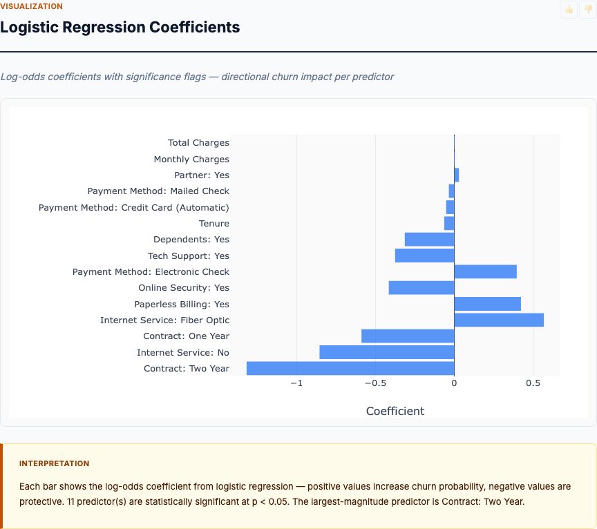
Regression Coefficients Table

This is the core output—raw regression coefficients with standard errors, t-statistics, p-values, and confidence intervals. Here's what each column reveals:

Coefficient: The estimated sales change per $1,000 increase in spend, controlling for other channels.

• Intercept (2.939): Expected sales when all channels spend $0. In practice, this is extrapolation—you never actually spend zero on all channels—so focus on the slope coefficients.
• TV (0.047): Each additional $1,000 in TV spend drives $47 in sales, holding Radio and Newspaper constant. ROI = 4.7%.
• Radio (0.189): Each additional $1,000 in Radio spend drives $189 in sales, controlling for TV and Newspaper. ROI = 18.9%.
• Newspaper (−0.001): Near-zero coefficient suggests no detectable effect. The negative sign is noise—p-value of 0.860 means not statistically significant.

Standard Error: Uncertainty in the coefficient estimate. TV's SE is 0.001, Radio's is 0.009, Newspaper's is 0.006. Smaller SE means more precise estimate. SE depends on sample size and residual variance—more data and less noise yield tighter estimates.

t-statistic and p-value: Tests the null hypothesis that the true coefficient is zero.

• TV: t = 32.8, p < 0.001. Reject the null. TV's effect is highly significant.
• Radio: t = 21.9, p < 0.001. Radio's effect is highly significant.
• Newspaper: t = −0.18, p = 0.860. Fail to reject the null. No evidence of a Newspaper effect.

Check the p-value. If p < 0.05, the coefficient is statistically significant at the 95% confidence level. That doesn't mean the effect is large or practically meaningful—just that it's unlikely to be zero. Combine significance with effect size: TV's coefficient is small (0.047) but highly significant and likely worthwhile at scale. Newspaper's coefficient is tiny and non-significant—no reason to believe it drives sales.

95% Confidence Interval: The range within which the true coefficient likely falls. TV's CI is [0.044, 0.049]—tight bounds, high precision. Radio's CI is [0.172, 0.206]. Newspaper's CI is [−0.013, 0.011], which crosses zero—consistent with no effect.

Wide CIs indicate low precision, often due to small sample size or high multicollinearity. Narrow CIs (like TV and Radio here) give you confidence in the point estimate.

Actual vs Predicted Sales

This scatter plot shows how well the regression model predicts sales. Each point represents one week: x-axis is actual sales, y-axis is predicted sales from the fitted model. The diagonal line is the ideal—perfect predictions fall exactly on it.

What you want to see: Points tightly clustered around the 45-degree line across the full range of sales. Here, the model performs well—R² is 0.897, meaning 89.7% of sales variance is explained by the three channels. Predictions are accurate from low-sales weeks (~$2K) to high-sales weeks (~$27K).

Red flags to watch for:

• Systematic underprediction at high spend: Points above the line at the right edge. Suggests diminishing returns—the linear model overestimates high-spend effectiveness. Consider adding quadratic terms (TV²) to model saturation.
• Systematic overprediction at low spend: Points below the line at the left edge. Suggests a threshold effect—channels don't work until spend exceeds a minimum. Consider piecewise regression or excluding very low-spend weeks.
• Increasing scatter at high spend: Heteroscedasticity—variance grows with spend level. Use robust standard errors or weighted least squares.

This plot shows none of those issues—residuals are evenly distributed around the line at all spend levels. That validates the linear model's functional form.

Practical implication: The model is reliable for predicting sales across your typical spend range. If you're considering a massive budget increase (e.g., 5x your historical max), extrapolation risk is high—the linear relationship may not hold. Incremental budget changes within your historical range? Safe to trust the coefficients.

Turning Regression Results Into Budget Decisions

You've read the report. Now what? Here's how to translate coefficients into action:

Step 1: Identify significant channels. TV and Radio have p < 0.001—definitely keep funding them. Newspaper has p = 0.860 and near-zero coefficient—cut it or test it in a controlled experiment before increasing spend.

Step 2: Calculate ROI per channel.

• TV: $0.047 return per $1 spent → 4.7% ROI
• Radio: $0.189 return per $1 spent → 18.9% ROI
• Newspaper: ~$0 return per $1 spent → 0% ROI

Radio delivers 4x the ROI of TV. Does that mean shift all budget to Radio? Not necessarily. Consider three factors:

1. Saturation: Radio's high ROI may reflect that you're currently underspending there. As you increase Radio spend, ROI may decline (diminishing returns). The linear model doesn't capture this—consider testing higher Radio budgets in a controlled experiment.
2. Reach: TV may have larger total reach even if per-dollar ROI is lower. If your goal is brand awareness, reach matters. If your goal is direct sales, ROI matters more.
3. Complementarity: TV and Radio may interact—TV builds awareness, Radio drives conversion. The regression assumes additive effects. If you suspect synergies, add interaction terms (TV × Radio) to the model.

Step 3: Allocate budget at the margin. The regression tells you which channel to increase next. If you have an extra $10K to spend, put it in Radio (18.9% ROI). Once Radio saturates or reaches competitive parity, TV becomes the next-best option (4.7% ROI). This is marginal analysis—allocate based on where the next dollar drives the most impact.

Step 4: Test your assumptions. Regression on observational data gives you correlations, not proven causation. Before reallocating millions, run a controlled experiment: randomize some markets to high Radio spend, others to current levels. Measure the difference. If the experimental lift matches the regression coefficient, you have causal confirmation. If not, investigate confounders the regression missed.

Common Pitfalls and How to Avoid Them

Pitfall 1: Confusing correlation with causation. Just because TV coefficient is 0.047 doesn't mean TV causes sales. It means TV and sales are associated after controlling for Radio and Newspaper. If you spent more on TV during holiday seasons (when sales are naturally high anyway), the coefficient conflates TV's true effect with seasonal demand. Solution: Add control variables (month, seasonality indicators) or run randomized tests.

Pitfall 2: Ignoring time lags. TV advertising might drive sales with a 2-week delay. The regression assumes spend and sales occur in the same week. If effects lag, coefficients are biased toward zero. Solution: Add lagged predictors (TV spend from 1 week ago, 2 weeks ago) or use distributed lag models.

Pitfall 3: Overfitting with too many predictors. If you add 20 channels with only 100 observations, the model will fit noise. Adjusted R² penalizes extra predictors—use it instead of raw R². Solution: Keep predictors ≤ sample size / 10 as a rough rule. Or use cross-validation to test out-of-sample prediction accuracy.

Pitfall 4: Extrapolating beyond your data range. The model predicts sales for spend levels you've observed. If your max historical TV spend is $300K and you plug in $1M, the prediction is pure guesswork. Diminishing returns likely kick in at high spend. Solution: Stay within historical ranges or fit non-linear models (polynomial, log) that capture saturation.

Pitfall 5: Assuming linearity. Real advertising often shows S-curves: no effect until a threshold, then rapid growth, then saturation. Linear regression misses this. Solution: Plot spend vs. sales to eyeball the functional form. If non-linear, use log transformations, polynomial terms, or specialized media mix models (adstock models with decay and saturation).

Pitfall 6: Ignoring interaction effects. TV might amplify Radio's effectiveness (synergy) or compete with it (cannibalization). Standard regression assumes effects add independently. Solution: Add interaction terms (TV × Radio) and test if they're significant. If the interaction coefficient is positive and significant, the channels synergize.

Advanced Extensions: When to Go Beyond Basic Regression

The three-channel linear regression shown here is a starting point. Real media mix modeling often requires additional sophistication:

Adstock models: Advertising has carryover effects—this week's TV ad influences next week's sales. Adstock models apply exponential decay to capture lagged impact. Instead of just TV spend this week, you model "effective TV exposure" = current spend + 0.5 × last week's spend + 0.25 × two weeks ago, etc. This better reflects how advertising builds and decays over time.

Saturation curves: Spend effectiveness declines at high budgets. A common form is diminishing returns: Sales = β × log(Spend). Or use Hill curves (S-shaped) to model both thresholds and saturation. These non-linear models require non-linear regression or transformation, but they capture reality better than straight lines.

Bayesian regression: Incorporate prior beliefs about channel effectiveness (from industry benchmarks or past campaigns) and update them with your data. Bayesian methods also quantify uncertainty more fully—you get probability distributions over coefficients, not just point estimates. Useful when sample size is small and you want to blend data with prior knowledge.

Hierarchical models: If you have data across multiple markets or products, fit a hierarchical model that estimates market-specific coefficients while borrowing strength from the overall average. This prevents overfitting to small markets and improves estimates for all.

Causal inference methods: If you can't randomize, use quasi-experimental designs like difference-in-differences (compare markets that increased TV to those that didn't) or regression discontinuity (if spend thresholds create natural experiments). These methods strengthen causal claims from observational data.

When should you use these advanced methods? When basic regression diagnostics fail (non-linear residual patterns, autocorrelation), when you have strong prior knowledge to incorporate, or when budgets are large enough that incremental accuracy justifies the modeling complexity.

Validating Your Model: Holdout Testing

How do you know the regression model will work on new data? Fit it on a training set (say, first 150 weeks) and test predictions on a holdout set (last 50 weeks). If training R² is 0.90 but holdout R² drops to 0.50, you've overfit.

For the example analysis, the full-sample R² is 0.897. In a proper validation, you'd expect holdout R² to be slightly lower (0.85-0.88) due to sampling variability. If it's much lower, simplify the model—remove non-significant predictors or reduce interaction terms.

Cross-validation is even better: split data into 5 folds, train on 4, test on 1, rotate through all folds. Average the test-set R² across folds for a robust estimate of out-of-sample performance. This is the gold standard for model validation when you can't run new experiments.

Integrating Regression Into Your Marketing Workflow

One-time regression analysis is useful. Continuous regression-driven optimization is powerful. Here's how to build it into your workflow:

Monthly refresh: Re-run the regression each month as new campaign data arrives. Track how coefficients change—if TV's ROI drops from 0.047 to 0.030, you may be saturating the channel or facing increased competition. Adjust budgets accordingly.

Automated alerts: Set thresholds—if any channel's p-value exceeds 0.05 (loses significance), flag it for review. If a previously non-significant channel becomes significant, test increasing its budget.

Budget optimizer: Feed regression coefficients into an optimization algorithm that maximizes predicted sales subject to your total budget constraint. This automates the allocation step: "Given $100K total budget and ROI of 4.7% (TV), 18.9% (Radio), 0% (Newspaper), how should I allocate?" The optimizer will load up on Radio until diminishing returns kick in, then shift to TV.

A/B testing integration: When regression suggests a high-ROI channel, validate it with a controlled test. Randomize some markets to high spend, measure the lift, compare to regression prediction. If they align, scale up with confidence. If they diverge, investigate what the regression missed (interaction effects, unobserved confounders).

Attribution modeling: Combine regression (for overall channel effectiveness) with user-level attribution (for individual customer journeys). Regression tells you TV drives $0.047 per dollar on average. Attribution tells you which customers saw TV ads before converting. Together, they paint a complete picture.

What This Analysis Does NOT Tell You

Be clear about the limits:

It doesn't tell you why a channel works. Radio's coefficient is 0.189, but is that because Radio ads are more persuasive? Because Radio reaches your target demographic better? Because Radio reminds people who saw TV ads? Regression is a black box—inputs and outputs, no mechanism. To understand why, run qualitative research or controlled experiments that isolate causal pathways.

It doesn't tell you which creative works. The analysis averages across all TV ads you ran. Some may have 10% ROI, others 2%, but you see the average 4.7%. To optimize creative, you need ad-level data and A/B tests of different messages, formats, and calls-to-action.

It doesn't predict what happens if you change strategy. The coefficients reflect historical spend patterns. If you suddenly shift from brand-building TV to direct-response TV, ROI may change. Regression assumes the future resembles the past. If your strategy or market shifts, re-estimate.

It doesn't account for external factors. Competitor actions, economic conditions, seasonality—if these aren't in the model, they're confounded with your channels. Add control variables (GDP, competitor spend, holiday indicators) to isolate your advertising effects from external shocks.

It doesn't guarantee profitability. TV's ROI is 4.7%. If your gross margin is 50% and customer lifetime value is high, 4.7% may be excellent. If your margin is 5%, you're losing money on every TV dollar. Combine regression ROI with your business economics to determine which channels are truly profitable.

FAQs: Advertising Spend Effectiveness Regression

What is the difference between correlation and causation in advertising analysis?

Correlation shows two variables move together—TV spend and sales both increased. Causation means one drives the other—TV spend actually causes sales lift. Multiple regression isolates each channel's independent effect by controlling for all other channels simultaneously, getting closer to causal estimates. But true causation requires randomized experiments where you control who sees which ads.

How do I know if my regression coefficients are statistically significant?

Check the p-value. If p < 0.05, the coefficient is statistically significant at the 95% confidence level—meaning there's less than a 5% chance you'd see an effect this large if the true effect were zero. Also examine the confidence interval: if it doesn't cross zero, the effect is significant. In the example, TV (p=0.000) and Radio (p=0.000) are highly significant; Newspaper (p=0.860) is not.

What does multicollinearity mean and why does it matter?

Multicollinearity means your advertising channels are correlated with each other—when TV spend goes up, Radio spend also tends to increase. This makes it harder to isolate each channel's independent effect. High multicollinearity inflates standard errors and makes coefficients unstable. Check the correlation matrix: correlations above 0.7-0.8 are concerning. The example shows moderate correlations (TV-Radio: 0.05, TV-Newspaper: 0.06), which is acceptable.

How large a sample do I need for media mix modeling?

Minimum 100-200 observations for stable coefficient estimates with 3 predictors. For detecting small effects (10-15% lift), you need 300+ observations. The sample dataset has 200 rows—adequate for detecting the medium-to-large effects observed (TV and Radio coefficients). If you're testing more channels or expect smaller effects, collect more data or run a longer campaign.

When should I use standardized coefficients instead of raw coefficients?

Use standardized coefficients to compare relative importance when channels use different scales. TV might be measured in thousands of dollars, Radio in hundreds. Standardized coefficients put everything in standard deviation units, making direct comparison valid. Use raw coefficients for budget decisions: "If I spend $1,000 more on Radio, I expect $189 in additional sales." Use standardized coefficients for strategy: "Radio has 2x the impact of TV per unit of variation."

Next Steps: From Analysis to Action

You've read the regression report. The coefficients point to Radio as the high-ROI channel, TV as moderate, Newspaper as ineffective. What now?

1. Validate with a controlled experiment. Randomize 20 markets to +50% Radio spend, 20 to current levels. Measure sales lift over 8 weeks. If experimental ROI matches regression estimate (18.9%), you have causal confirmation. Scale up with confidence.

2. Model non-linearity. The regression assumes constant ROI—each Radio dollar drives $0.189 regardless of total spend. Reality: ROI likely declines at high spend (saturation). Fit a log or polynomial model to capture diminishing returns. Use it to find the optimal Radio budget where marginal ROI equals your hurdle rate.

3. Add control variables. Include seasonality (month dummies), competitor actions (if you have data), economic indicators (consumer confidence). This isolates advertising effects from external factors and improves coefficient accuracy.

4. Test interactions. Does TV amplify Radio's effectiveness? Add a TV × Radio interaction term. If significant and positive, the channels synergize—coordinate campaigns for maximum impact.

5. Optimize budget allocation. Use the coefficients to simulate different budget scenarios. Build a simple optimizer that maximizes predicted sales subject to your total budget. Run it monthly as coefficients update.

6. Measure long-term effects. Current-week spend may drive next-quarter sales (lagged effects). Add lagged predictors to capture long-term ROI. Some channels (brand-building TV) show delayed impact that immediate regression misses.

Before you draw conclusions, let's check the experimental design. Or in this case, let's run the experiment to validate the observational regression. That's the difference between correlation and causation—and it's the difference between guessing which channels work and knowing for certain.

Related Articles