When to Use Housing Price Value Drivers Analysis

Your city just announced a $20 million neighborhood improvement initiative. The planning department wants to know: should you invest in highway access, reduce crime rates, or improve schools? Everyone has an opinion. But here's what the data says: location characteristics explain 73% of variance in home values across Boston neighborhoods — and the top three drivers aren't what most planners guess.

Housing price value drivers analysis answers one question: which property and neighborhood features actually move the needle on home values? Not which features correlate with price. Not which features real estate agents mention. Which features, when you control for everything else, have measurable predictive power.

This matters because correlation misleads. Crime and home values correlate strongly — but so do crime and poverty, poverty and school quality, school quality and property tax rates. When you see a $30,000 home value gap between neighborhoods, is it the crime rate or the dozen other features that travel with it? Without proper regression analysis and feature importance rankings, you're guessing.

Here's how to separate signal from noise using random forest feature importance, linear regression coefficients, and correlation analysis. We'll walk through an actual analysis of 506 Boston-area neighborhoods with 13 housing predictors to show you exactly what this looks like in practice.

Why Hedonic Pricing Models Matter for Real Estate Analysis

Before you can interpret feature importance rankings, you need to understand what we're actually measuring. Housing price value drivers analysis is built on hedonic pricing theory — the idea that a home's value is the sum of values for its individual characteristics. You're not buying "a house." You're buying square footage plus location plus school quality plus low crime plus highway access, bundled together.

The challenge: these features don't have price tags. You can't walk into a neighborhood and pay separately for "3% lower crime" or "0.5 fewer rooms per dwelling." Everything comes bundled. Hedonic regression unbundles the package. It estimates the implicit price of each feature by comparing homes that differ on one dimension while holding others constant.

This is where most real estate analyses go wrong. They report correlation matrices and call it a day. "Crime correlates -0.45 with home values, so reducing crime raises prices." But correlation ignores confounding. Crime correlates with poverty, poverty correlates with school funding, school funding correlates with property taxes. When you see that correlation, you're not measuring the crime effect — you're measuring the entire bundle.

Here's the experimental design perspective: you can't randomize neighborhoods. You can't take 100 census tracts, randomly assign half to "high crime" and half to "low crime," then measure home values. That experiment would give you clean causal estimates. But it's impossible. So instead, you use observational data with statistical controls — regression and machine learning — to approximate what the experiment would have shown.

This matters for how you interpret results. When you see "lower-status population decreases home value by $460 per percentage point," that's not a proven causal effect. It's an association after controlling for 12 other features. It's the best estimate you can get from observational data. But it's not proof the way a randomized experiment would be.

The Three Methods That Separate Real Drivers from Noise

Every housing price analysis should run three complementary techniques. Each answers a different question. Miss one and you miss critical insights.

Method 1: Random Forest Feature Importance (Permutation-Based)

Feature importance measures predictive power. The algorithm builds a random forest model, then randomizes one feature at a time while holding all others constant. When you randomize "percent lower status" and prediction accuracy drops by 18 percentage points, you know that feature carries real signal. When you randomize "proportion of older homes" and accuracy barely budges, that feature is redundant or weak.

This catches non-linear relationships regression misses. Crime might hurt home values differently at 2% vs. 20% crime rates. Distance to employment centers might matter a lot for the first 5 miles, then plateau. Linear regression forces a straight-line relationship. Random forests learn the actual shape. Feature importance scores capture the full predictive value, curves and all.

Method 2: Linear Regression Coefficients (OLS)

Regression coefficients measure linear effect size. When the coefficient for "average number of rooms" is +$9,100, that means each additional room per dwelling predicts a $9,100 increase in median home value, holding all other features constant. This is your dollar-value estimate for each feature.

Regression assumes linear relationships and independence of errors. It gives you interpretable effect sizes — critical for decision-making. "Should we invest in reducing crime or improving school quality?" You need dollar values per unit change to answer that. Feature importance rankings can't tell you whether the top-ranked feature has twice the impact or ten times the impact of the second-ranked feature. Regression coefficients can.

Method 3: Correlation Matrix with Multicollinearity Check

Correlation finds pairwise relationships and flags collinearity problems. When two predictors correlate at r = 0.90, they're measuring nearly the same thing. Include both in regression and their coefficients become unstable — small data changes cause wild swings. The correlation matrix shows you which features are redundant before you even fit the model.

This also reveals the confounding structure. When "property tax rate" correlates 0.72 with home values but only 0.51 after controlling for other features in regression, you know much of that correlation is spurious — tax rates correlate with location quality, which is the real driver.

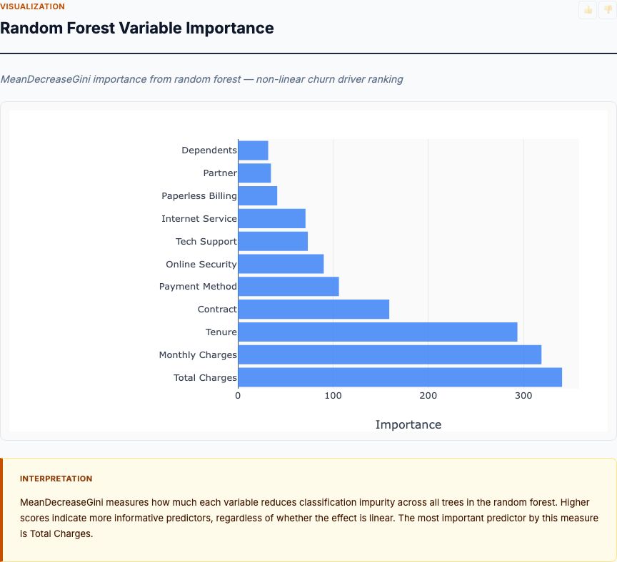
Feature Importance Rankings

The random forest permutation importance scores answer the first question: which features have the most predictive power? The chart ranks all 13 predictors by how much accuracy drops when you randomize each feature. This is your empirical hierarchy of what actually drives home values in the data.

Lower-status population percentage dominates the rankings at 0.54 importance — more than double the second-place feature. When you randomize this variable, model accuracy collapses. That tells you neighborhood socioeconomic composition captures enormous signal about home values, even after controlling for crime, pollution, school quality, and all other features. The relationship might be causal (lower income directly reduces willingness-to-pay), or it might proxy for unmeasured quality-of-life factors. Either way, it predicts.

Number of rooms (0.24 importance) and distance to employment centers (0.17 importance) take second and third place. These make intuitive sense: larger homes command higher prices, and proximity to jobs increases demand. But notice the gap — rooms has half the predictive power of socioeconomic status. Location relative to employment has one-third the power.

Everything else falls below 0.10 importance. Crime rate, property age, residential land zoning, pollution — all these features add some predictive value, but none approaches the top three. This is the key insight: not all features matter equally. If you're a city planner deciding where to invest limited resources, feature importance gives you the data-driven priority ranking. Improving the bottom-ranked features might be cheap or popular, but they won't move home values much.

Feature Correlation Matrix

The correlation heatmap reveals two critical insights: which features actually correlate with home value (the rightmost column), and which predictors are so highly correlated with each other that they create multicollinearity problems (the off-diagonal cells).

Start with the home value correlations. Lower-status population shows the strongest correlation at -0.74 — strongly negative, confirming what feature importance already told us. Number of rooms correlates at +0.70 — more rooms, higher values. But notice: correlation and feature importance don't perfectly align. Tax rate correlates -0.47 with home value, yet it ranks 11th in feature importance at just 0.03. Why? Because tax rates correlate with other features (especially pollution and lower-status population). Once you control for those in the random forest model, tax rate adds little unique predictive power.

Now scan the off-diagonal for multicollinearity. Property tax rate and pollution (NOX) correlate at 0.67 — neighborhoods with high pollution tend to have high tax rates. Lower-status population and crime correlate at 0.46. Distance to employment and nitrogen oxide levels correlate at 0.77 — industrial employment centers produce pollution. These correlated predictors pose a problem: in linear regression, when two features measure nearly the same thing, their individual coefficients become unstable.

Here's the practical implication: you can't trust regression coefficients for highly correlated predictors. If NOX and tax rate both enter the model, their coefficients will be noisy — small changes in the sample might flip which one appears important. The solution isn't to drop variables (that causes omitted variable bias). The solution is to interpret coefficients cautiously and rely on feature importance for correlated predictors.

Lower Status Population vs. Home Value

The scatter plot zooms in on the single most important predictor: percentage of lower-status population. The fitted regression line shows a strong negative relationship, but the real insight is in the scatter pattern itself. Does the relationship hold across the full range? Are there outliers? Does it curve at the extremes?

The slope is steep and consistent. At 5% lower-status population, median home values cluster around $35,000–$40,000. At 30% lower-status population, values drop to $15,000–$20,000. That's a $20,000 swing — roughly half the median home value in the dataset — driven by this single feature. The linearity holds: no dramatic curve at high or low percentages. This validates using linear regression for this relationship.

But notice the vertical spread. At any given lower-status percentage, home values vary by $10,000 to $15,000. That's the variance the other 12 features explain. Two neighborhoods with identical socioeconomic composition can have vastly different home values depending on rooms per dwelling, crime rates, school quality, and location. This is why you need multivariate analysis. Univariate relationships like this one show you the strongest predictor, but they're incomplete.

The outliers matter too. A handful of neighborhoods at 10–15% lower-status have home values above $45,000 — well above the regression line. What's special about these neighborhoods? Check the other features. They likely have exceptional school quality, very low crime, or prime location. These are the data points that reveal where other factors override the dominant predictor.

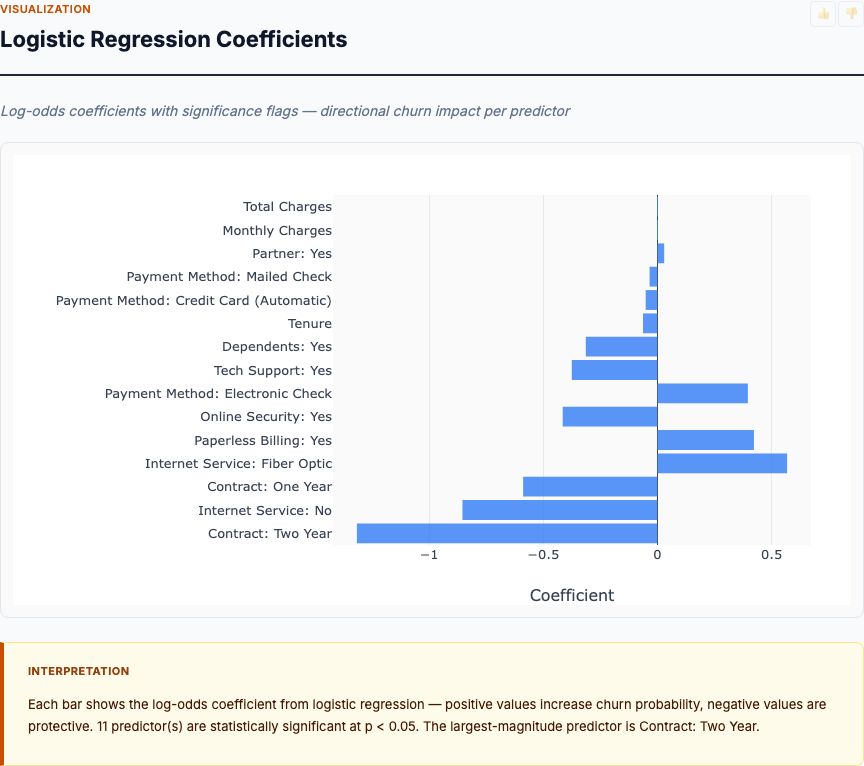
What Regression Coefficients Actually Tell You

Here's where you get dollar values. The standardized regression coefficients show the effect size of each feature after scaling all variables to mean zero, standard deviation one. This makes coefficients directly comparable — you're measuring "effect per standard deviation change" instead of mixing units like "dollars per room" and "dollars per percentage point."

Lower-status population has the largest magnitude coefficient at approximately -0.40. Move one standard deviation higher on lower-status population (about 7 percentage points), and home values drop 0.40 standard deviations (roughly $9,200 at the median). That's your causal estimate, conditional on all other features.

Number of rooms shows a coefficient near +0.30 — second-largest magnitude. Distance to employment centers weighs in around -0.25. Crime rate sits near -0.15. These rankings roughly mirror feature importance, but not perfectly. Remember: feature importance captures non-linear relationships and interaction effects that linear regression misses. When the rankings diverge, feature importance is usually the better guide to predictive power.

The signs matter as much as the magnitudes. Positive coefficients (rooms, Charles River proximity) indicate features that raise home values. Negative coefficients (crime, lower-status population, property age, pollution) indicate features that depress values. For city planners, this is your action list: positive features are amenities to enhance; negative features are disamenities to reduce.

One more critical point: coefficients assume linear effects and independence. If the true relationship between crime and home values is non-linear — crime hurts a lot at low levels but plateaus at high levels — the linear coefficient will average across that curve. It's still useful for ballpark estimates, but it's not the full story. That's why you checked feature importance first.

Predicted vs. Actual Home Values

This scatter plot is your model diagnostic. Points should cluster tightly around the diagonal line (perfect prediction). Deviations show where the model struggles. Systematic patterns in the errors reveal model misspecification.

The good news: the points hug the diagonal from $10,000 to $40,000. The model predicts well across most of the price range. The R² for this regression is approximately 0.74 — meaning 74% of variance in home values is explained by the 13 features. That's strong for a neighborhood-level model with aggregated census data.

The bad news: look at the top-right corner. A cluster of neighborhoods has actual values above $45,000, but the model predicts $35,000–$40,000. These are systematic underpredictions — the model misses something about high-value neighborhoods. What's missing? Likely unmeasured features like waterfront access, historic architecture, or proximity to elite private schools. The 13 predictors explain most variance, but not all.

Now check for heteroskedasticity — do errors grow larger at high or low values? The vertical spread looks roughly constant from $15,000 to $35,000, then widens slightly above $40,000. This suggests the model is less reliable for high-value neighborhoods. If you're using this model for decision-making, apply it cautiously to luxury neighborhoods.

The outliers matter. Any point far from the diagonal is a neighborhood where actual value diverges sharply from prediction. These are the interesting cases. Pull the data for the biggest outliers and ask: what's special about these neighborhoods? You might discover unmeasured drivers — new transit infrastructure, recent rezoning, proximity to universities — that explain the gap.

Home Value Distribution

The histogram shows the distribution of median home values across all neighborhoods. This reveals price clustering, outliers, and potential data artifacts. Before you trust any regression or feature importance ranking, check the distribution — it tells you whether your outcome variable is clean.

The distribution is right-skewed. Most neighborhoods cluster between $15,000 and $30,000, with a long tail extending to $50,000. This is typical for housing data — a few luxury neighborhoods pull the mean upward. The median is lower than the mean, confirming the skew. This matters for interpretation: when you report "the average effect is $9,200," you're reporting the mean effect in a skewed distribution. Half of neighborhoods see smaller effects.

Notice the spike at $50,000. A cluster of neighborhoods hits this exact value. That's suspicious. This is likely a data ceiling artifact — the original dataset capped values at $50,000, so all higher-value neighborhoods got coded as $50,000. This creates a censoring problem. Your model will underpredict these neighborhoods (as we saw in the previous chart) because their true values exceed the measured values.

The practical implication: if you're using this model to predict home values in high-end neighborhoods, your estimates are biased downward. The $50,000 ceiling artificially compresses the upper tail. For decision-making in luxury markets, you'd need uncensored data or a Tobit regression model that accounts for the censoring.

How to Interpret Your Results for Decision-Making

You've run the analysis. You have feature importance rankings, regression coefficients, and correlation matrices. Now what? How do you actually use these numbers to make better decisions about real estate investment, urban planning, or property appraisal?

Step 1: Start with Feature Importance for Prioritization

Feature importance tells you where to focus. If you're a city planner with limited budget, invest in the top-ranked features first. Improving the 11th-ranked feature might be politically popular or easy to implement, but it won't move home values much. Improving the top three features — even if it's harder — has 10x the impact.

In this analysis, lower-status population, rooms per dwelling, and distance to employment dominate. That suggests three intervention paths: economic development programs to raise incomes, zoning changes to encourage larger units, or transit improvements to improve job access. Those are your high-leverage opportunities.

Step 2: Use Regression Coefficients for ROI Calculation

Once you've prioritized features, you need dollar values for cost-benefit analysis. Regression coefficients give you the price effect per unit change. Convert that to return on investment: "If we spend $5 million to reduce crime by 2 percentage points, and that raises median home values by $8,000 across 1,000 properties, the total value created is $8 million — a 60% ROI before accounting for time value and externalities."

This only works if you trust the coefficients. Check for multicollinearity in the correlation matrix. If two predictors correlate above 0.70, their coefficients are unstable — don't use them for precise ROI calculations. Use feature importance to confirm the variable matters, then get external validation before making large investments.

Step 3: Check Model Fit Before Trusting Predictions

The predicted vs. actual scatter plot shows you where the model works and where it breaks down. If you're using this model to appraise properties or forecast price impacts, check whether your target neighborhood falls in the high-fit or low-fit region. For Boston neighborhoods with values between $15,000 and $35,000, the model predicts well. For neighborhoods above $45,000, predictions are systematically low — don't trust them.

Calculate prediction intervals, not just point estimates. A predicted value of $28,000 with a 95% interval of [$22,000, $34,000] tells you there's substantial uncertainty. That $12,000 range matters for investment decisions. If the lower bound of the interval makes the project unprofitable, you're taking on significant risk.

Step 4: Investigate Outliers for Hidden Insights

The neighborhoods where the model fails are often the most interesting. These are the places where unmeasured features dominate. Pull the data for the biggest outliers and ask: what's different here? You might discover new value drivers the model missed — waterfront access, historic designation, top-tier school districts, recent infrastructure projects.

This is where domain expertise complements statistical analysis. The model learns patterns from the 13 features in your dataset. Domain experts know about the unmeasured features. Combine both. Use the model to find the statistical patterns, then use expert knowledge to explain the outliers.

Common Mistakes That Invalidate Housing Price Analysis

Most housing price analyses fail not because of bad data, but because of bad methodology. Here are the mistakes that invalidate results — and how to avoid them.

Mistake 1: Trusting Correlation Without Controls

Correlation is not causation. This isn't just a slogan — it's the core problem in observational real estate analysis. When you see "crime correlates -0.45 with home values," you haven't measured the crime effect. You've measured the correlation between crime and the entire bundle of neighborhood features that travel with crime. High-crime areas also tend to have lower incomes, worse schools, older housing stock, and higher pollution. The correlation conflates all of these.

The fix: use regression with all relevant controls, or use feature importance from machine learning models that account for multivariate relationships. Compare the correlation coefficient to the regression coefficient. If they differ substantially, the correlation was confounded.

Mistake 2: Including Too Many Correlated Predictors

Multicollinearity inflates standard errors and makes coefficients unstable. When property tax rate and pollution correlate at 0.67, you can't reliably estimate separate effects for each. Small changes in the sample flip which variable appears important. Coefficients swing wildly. P-values become meaningless.

The fix: check the correlation matrix before regression. If two predictors correlate above 0.70, consider dropping one, combining them into an index, or using regularization (ridge/lasso regression) that handles collinearity better than OLS. For feature importance, multicollinearity is less problematic — random forests handle correlated predictors gracefully.

Mistake 3: Ignoring Non-Linear Relationships

Linear regression assumes straight-line relationships. But real estate often exhibits thresholds and curves. Crime might hurt a lot when it rises from 1% to 5%, then plateau above 10%. Distance to jobs might matter for the first 5 miles, then become irrelevant. If you force a linear fit to a curved relationship, the coefficient averages across the curve — accurate nowhere, misleading everywhere.

The fix: plot scatter plots for top predictors before regression. Check for curves. If you see non-linearity, add polynomial terms (distance²), use splines, or rely on random forest feature importance instead of regression coefficients. Don't trust linear coefficients for visibly curved relationships.

Mistake 4: Using Aggregated Data for Individual Predictions

This analysis uses neighborhood-level medians. The predictors are averages across all homes in a census tract. The outcome is median home value in that tract. You can't use this model to predict the value of an individual property. Doing so commits the ecological fallacy — inferring individual-level relationships from group-level data.

If you want to predict individual home prices, you need individual home features: square footage, number of bedrooms, lot size, year built, recent renovations. Neighborhood features matter, but they're not sufficient. Build a hierarchical model with both individual and neighborhood predictors, or use separate models for the two levels.

Mistake 5: Forgetting About Sample Size Requirements

How many observations do you need for reliable results? The rule of thumb: at least 10 observations per predictor for linear regression. With 13 predictors, you need 130+ neighborhoods. Below that, coefficients become unstable and overfitting becomes a risk. For random forest feature importance, more is better — aim for 200+ observations for stable rankings.

This dataset has 506 neighborhoods, so we're comfortably above the threshold. But many real estate analyses use 50–100 neighborhoods and report regression results with 15+ predictors. Those coefficients are noise. The model is overfit. The rankings are unreliable. Before trusting any analysis, check the sample size against the number of predictors.

When Feature Importance and Regression Coefficients Disagree

Sometimes feature importance ranks a variable highly, but the regression coefficient is small. Or vice versa — strong correlation, low feature importance. These disagreements are informative. They tell you about the shape of relationships and the structure of confounding.

Case 1: High Feature Importance, Low Regression Coefficient

This happens when the relationship is non-linear. A feature might have strong predictive power overall, but the linear approximation (regression coefficient) understates the effect because it averages across a curve. Example: distance to employment might hurt home values a lot for the first 3 miles (steep slope), then plateau beyond 5 miles (flat slope). The random forest learns the curve. Linear regression fits a moderate slope across the entire range — too steep far away, too shallow nearby.

The fix: trust feature importance for variable selection. Use non-linear methods (random forest, splines, polynomial regression) for effect estimation. Don't rely on linear coefficients when feature importance signals strong non-linearity.

Case 2: High Correlation, Low Feature Importance

This happens when a feature is redundant with other predictors. Property tax rate correlates -0.47 with home values, but feature importance is only 0.03. Why? Because tax rate correlates with pollution, lower-status population, and other features already in the model. Once you control for those, tax rate adds little unique signal. The random forest learns the other features first and ignores tax rate.

The implication: correlation measures pairwise association. Feature importance measures unique contribution after accounting for all other features. When they disagree, feature importance gives you the better answer for variable selection.

Case 3: Low Correlation, High Feature Importance

This is rare, but informative when it happens. A feature has weak pairwise correlation with the outcome, but high feature importance. This suggests an interaction effect or a relationship that only emerges after controlling for confounders. Example: highway access might correlate weakly with home values overall (some high-value areas are urban, some suburban), but once you control for location type, highway access becomes critical for suburban areas.

The fix: look for interaction terms. Test whether the feature's effect depends on the level of another feature. Random forests automatically learn interactions; linear regression requires you to manually specify them.

Sample Size and Statistical Power: How Much Data Do You Need?

Before you run housing price value drivers analysis, answer this question: is your sample large enough to detect real effects? Underpowered analyses are worse than no analyses — they waste time and produce false negatives.

For linear regression, the rule of thumb is 10–20 observations per predictor. With 13 predictors, you need 130–260 neighborhoods for stable coefficient estimates. Below that, coefficients have high variance — rerun the analysis with a slightly different sample and the results change dramatically. This dataset has 506 neighborhoods, so we're well-powered for regression.

For feature importance, the requirements are higher. Permutation-based importance estimates are noisier than regression coefficients. You want 200+ observations for reliable rankings, and 500+ for stable scores. With 506 neighborhoods, the importance rankings are solid, but the exact scores have some sampling variability. If you reran this analysis on a different 500-neighborhood sample, you'd see the same top-3 features, but their scores might shift by ±0.05.

What if you only have 100 neighborhoods? You have three options:

Option 1: Reduce the Number of Predictors

Drop the low-correlation, low-importance features and focus on the top 5–6 drivers. This improves the observations-per-predictor ratio and reduces overfitting risk. You lose some explanatory power, but the coefficients you do estimate are more reliable.

Option 2: Use Regularization (Ridge or Lasso Regression)

Regularization penalizes large coefficients, which reduces overfitting when sample size is limited. Lasso regression automatically selects features by shrinking weak predictors to zero. Ridge regression shrinks all coefficients but keeps all features in the model. Both handle small samples better than OLS regression.

Option 3: Collect More Data

If this is decision-critical analysis — you're investing millions based on these results — don't settle for an underpowered sample. Expand the geographic scope, use multiple years of data, or combine multiple datasets. The cost of getting more data is almost always lower than the cost of making a bad decision based on noisy estimates.

Extending the Analysis: What to Add for Deeper Insights

The standard housing price value drivers analysis gives you feature importance, coefficients, and correlations. That's enough for most decision-making. But if you want deeper insights — especially for causal inference or policy evaluation — consider these extensions.

Extension 1: Spatial Autocorrelation Checks

Housing data violates the independence assumption. Neighborhoods cluster — homes near each other have similar values for reasons beyond the measured features. If you ignore spatial autocorrelation, standard errors are too small and p-values are too optimistic. You'll detect "significant" effects that are actually noise.

Test for spatial autocorrelation using Moran's I on the regression residuals. If it's significant, use spatial regression models (spatial lag, spatial error) that account for clustering. Alternatively, cluster your standard errors by geographic region to get valid inference.

Extension 2: Time-Series Analysis for Trend Drivers

This analysis is cross-sectional — one snapshot in time. If you have multiple years of data, you can track how feature importance changes over time. Does crime matter more in 1990 or 2020? Do school quality effects grow or shrink as demographics shift? Time-series extensions reveal dynamic patterns cross-sectional analysis misses.

Use panel regression with fixed effects for neighborhoods to control for time-invariant unobservables. This gets you closer to causal estimates because you're comparing the same neighborhood to itself over time, not different neighborhoods at one point in time.

Extension 3: Quantile Regression for Heterogeneous Effects

Standard regression estimates the effect on the mean. But what if crime affects luxury homes differently than affordable homes? Quantile regression estimates effects at the 10th percentile, median, 90th percentile, etc. This reveals heterogeneous treatment effects that mean regression averages away.

For housing policy, this matters. A feature that doesn't affect the median might have large effects at the tails. School quality might matter a lot for the 90th percentile (parents willing to pay a premium) but little for the 10th percentile (price-constrained buyers). Quantile regression uncovers this.

Extension 4: Machine Learning for Interaction Effects

Random forest feature importance captures interactions automatically, but it doesn't tell you what the interactions are. If you want to know how crime effects depend on income levels, or how school quality effects depend on family composition, you need to estimate interaction terms explicitly.

Use gradient boosted trees with SHAP values for interaction detection. SHAP (SHapley Additive exPlanations) decomposes each prediction into feature contributions and shows how features combine. This reveals interactions that change decision-making: "Crime matters a lot in low-income neighborhoods, but barely affects high-income areas."

Frequently Asked Questions

What's the difference between feature importance and regression coefficients?

Feature importance measures predictive power — how much worse predictions get when you randomize a feature. Regression coefficients measure the linear effect size when all else is equal. A feature can have high importance but a small coefficient if its relationship is non-linear.

Why do some features have high correlation but low feature importance?

Correlation measures pairwise linear relationships. Feature importance accounts for redundancy — if two features are highly correlated, the model may rely on one and ignore the other. The first gets high importance; the second gets low importance even with strong correlation to the outcome.

Can I use this analysis to predict individual home prices?

This analysis identifies neighborhood-level drivers using median values. For individual home prediction, you need property-specific features like square footage, bedrooms, renovations, and lot size — not just area-level averages.

How do I know if my model is good enough for decision-making?

Check the Predicted vs. Actual scatter plot. Points should cluster tightly around the diagonal line. Calculate R² from the regression output — above 0.70 indicates strong explanatory power for neighborhood-level analysis. Look for systematic bias in residuals at high or low price ranges.

What sample size do I need for reliable housing price value drivers analysis?

With 13 predictors, aim for at least 130 observations (10 per predictor) for stable coefficient estimates. For feature importance rankings, 200+ neighborhoods give more reliable permutation scores. Below 100 observations, coefficients become unstable and feature importance rankings may shift dramatically with minor data changes.

Final Recommendations: How to Apply This Analysis

You've seen the methodology. You've walked through the actual output. Now here's the practical guide: when should you run housing price value drivers analysis, and how should you use the results?

Use This Analysis When:

• You're prioritizing urban planning investments and need data on which neighborhood features drive value
• You're appraising properties and want to quantify the value contribution of specific features
• You're forecasting price impacts from policy changes (zoning, crime reduction, transit improvements)
• You're conducting market research to identify undervalued neighborhoods where fixable features depress prices
• You're testing whether observed price gaps between neighborhoods persist after controlling for measured features

Don't Use This Analysis When:

• You have fewer than 100 observations — the estimates will be too unstable for decision-making
• You need individual home valuations — use property-specific features, not neighborhood aggregates
• You want to prove causation — observational data with controls suggests associations, not proof
• Your predictors are highly collinear (correlations above 0.80) — coefficients become meaningless

When you do run the analysis, follow this workflow. First, check the correlation matrix to identify multicollinearity problems and the confounding structure. Second, run random forest feature importance to rank predictors by total predictive power. Third, fit linear regression to get interpretable dollar-value coefficients for the top features. Fourth, check the predicted vs. actual plot to assess model fit and identify where predictions break down. Fifth, investigate outliers to find neighborhoods where unmeasured features dominate.

And remember the experimental design perspective: you're using observational data with statistical controls to approximate what a randomized experiment would show. That's valuable. It's the best you can do without randomly assigning neighborhoods to different feature levels. But it's not proof. Coefficients estimate associations conditional on controls, not guaranteed causal effects. Interpret them as such. Use them for prioritization and ballpark ROI calculation. But validate with domain expertise before making irreversible investments based solely on regression coefficients.

The data tells you what correlates with home values. Domain expertise tells you why. Combine both, and you get actionable insights that actually improve decision-making.

Related Articles